SEAA 4243 · 2D Heat Transfer

StartMula

What to doApa perlu dibuat Follow the plan: before class, in class, after class. Each item links to where it is done and ticks itself when it is. Continue takes you to the first thing not yet done.Ikut pelan: sebelum kelas, dalam kelas, selepas kelas. Setiap item dipautkan ke tempat ia dibuat dan ditanda sendiri apabila selesai. Sambung membawa anda ke perkara pertama yang belum selesai.

Counts toward progress:Dikira dalam kemajuan: the bar averages six parts equally: Notes, Slides, Examples, Exercises, Explorer and the can-do checklist. Each tab’s badge shows its own count.bar ini purata enam bahagian secara sama rata: Nota, Slides, Contoh, Latihan, Explorer dan senarai semak boleh-buat. Lencana pada setiap tab menunjukkan kiraannya sendiri.

Your planPelan anda

Before classSebelum kelas≈ 17 min

Read Notes §1 (9 min)Baca Nota §1 (9 min)
Recall question 1 (on this page)Soalan ingat semula 1 (di halaman ini)
Recall question 2 (on this page)Soalan ingat semula 2 (di halaman ini)

In classDalam kelas3 h · 6 activities3 jam · 6 aktiviti

A1 the boundary term · A2 [k] and {q}A1 boundary term · A2 [k] dan {q}
A3 connectivity · A4 assembly · A5 verificationA3 connectivity · A4 assembly · A5 pengesahan
A6 temperature at (0.3, 0.2) mA6 temperature pada (0.3, 0.2) m
QR Explorer: Heat Conduction Explorer, task 1Explorer QR: Heat Conduction Explorer, tugasan 1

After classSelepas kelas≈ 110 min

Notes §1–§6 (50 min)Nota §1–§6 (50 min)
Slides, all 45Slides, kesemua 45
Worked examples (3)Contoh bekerja (3)
Exercises A, B, C (~35 min)Latihan A, B, C (~35 min)
Explorer tasks 1–4Tugasan Explorer 1–4
Can-do checklistSenarai semak boleh-buat

○ to do · ✓ done · – done in class, not tracked. Click an item to go to it.○ belum · ✓ selesai · – dibuat dalam kelas, tidak dijejak. Klik item untuk pergi kepadanya.

What this part coversApa yang bahagian ini liputi

Part 1 gave the PDE and the element; this part turns them into numbers. The Galerkin weighted residual and integration by parts give [k]{T̂}ᵀ = {q} + {b}; the element matrices are evaluated in closed form, assembled through a connectivity table, the known temperatures are imposed, and the text’s plate is solved by hand and checked against a refined mesh. Plane stress reuses every one of these steps with two unknowns per node.Part 1 memberi PDE dan element; bahagian ini menukarkannya kepada nombor. Galerkin weighted residual dan integration by parts memberi [k]{T̂}ᵀ = {q} + {b}; matrix element dinilai dalam closed form, di-assemble melalui connectivity table, temperature yang diketahui dikenakan, dan plat dalam teks diselesaikan secara tangan dan disemak dengan mesh yang di-refine. Plane stress menggunakan semula setiap langkah ini dengan dua unknown setiap node.

After this part you should be able toSelepas bahagian ini, anda sepatutnya boleh

Apply the Galerkin weighted residual method and integration by parts to obtain [k]{T̂}ᵀ = {q} + {b} and explain what each term means.Menggunakan Galerkin weighted residual method dan integration by parts untuk memperoleh [k]{T̂}ᵀ = {q} + {b} dan menerangkan maksud setiap term.
Evaluate the conductance matrix [k] and the load vectors {q} and {b} of a 4-node rectangular element in closed form.Menilai conductance matrix [k] dan load vector {q} dan {b} bagi 4-node rectangular element dalam closed form.
Assemble element matrices into the global system with a connectivity table and impose Dirichlet conditions by row–column elimination.Meng-assemble matrix element ke dalam sistem global dengan connectivity table dan mengenakan Dirichlet condition melalui row–column elimination.
Solve a small problem by hand, post-process temperature and flux at a point, and judge the result against a refined mesh.Menyelesaikan masalah kecil secara tangan, post-process temperature dan flux pada satu titik, dan menilai hasilnya berbanding mesh yang di-refine.

Text: Mohd Yassin et al., Two-Dimensional Finite Element Formulations for Heat, Solids and Fluids (with Matlab), MSNM 2020, §2.2.2–§2.4.Teks: Mohd Yassin et al., Two-Dimensional Finite Element Formulations for Heat, Solids and Fluids (with Matlab), MSNM 2020, §2.2.2–§2.4.

Recall from Part 1Ingat semula Part 1

Two questions before class. Not graded; one try each.Dua soalan sebelum kelas. Tidak bergred; satu cubaan setiap satu.

Recall 1Ingat semula 1

The boundary condition that needs no action in the finite element model isBoundary condition yang tidak memerlukan tindakan dalam model finite element ialah

Recall 2Ingat semula 2

N₂ = x(b − y)/(ab) at node 3, (a, b), equalsN₂ = x(b − y)/(ab) pada node 3, (a, b), bersamaan

Can-do checklistSenarai semak boleh-buat

Rate yourself after the exercises. “Without notes” is the exam condition and counts in full; “With notes” counts half.Nilai diri anda selepas latihan. “Tanpa nota” ialah keadaan peperiksaan dan dikira penuh; “Dengan nota” dikira separuh.

Write the weighted residual, integrate by parts, and name [k], {q} and {b}.Menulis weighted residual, integrate by parts, dan menamakan [k], {q} dan {b}.

Compute s₁…s₄ for any a, b, k_x, k_y and check a row.Mengira s₁…s₄ untuk sebarang a, b, k_x, k_y dan menyemak satu baris.

Assemble a small mesh from a connectivity table and impose known temperatures.Meng-assemble mesh kecil daripada connectivity table dan mengenakan temperature yang diketahui.

Convert a global point to local coordinates and interpolate T and the flux.Menukar titik global kepada koordinat local dan interpolate T serta flux.

Files and settingsFail dan tetapan

Open the Explorer in a new tabBuka Explorer dalam tab baharu Course home · export or import progressLaman kursus · export atau import kemajuan

Progress is stored in this browser only. It is your own record, not a gradebook; graded work stays in eLearning.Kemajuan disimpan dalam pelayar ini sahaja. Ia rekod anda sendiri, bukan buku gred; kerja bergred kekal di eLearning.

NotesNota

What to doApa perlu dibuat Read each section, answer its Quick check (not graded, one try), then tick “Mark this section as read” at the end of the section. “Key points only” is the revision view.Baca setiap seksyen, jawab Semak cepat di dalamnya (tidak bergred, satu cubaan), kemudian tanda “Tanda seksyen ini sudah dibaca” di hujung seksyen. “Perkara utama sahaja” ialah paparan ulang kaji.

Counts toward progress:Dikira dalam kemajuan: sections ticked as read.seksyen yang ditanda sudah dibaca.

Equation numbers follow the text.Nombor persamaan mengikut teks.

1. Galerkin and integration by partsGalerkin dan integration by parts

≈ 9 min

Substitute the approximation T = {N}{T̂}ᵀ of Part 1 into the PDE and it does not balance: a bilinear field cannot satisfy a second-order equation at every point. The residual is what is left over. Four unknowns T̂₁…T̂₄, one equation, and it holds nowhere exactly.Gantikan approximation T = {N}{T̂}ᵀ dari Part 1 ke dalam PDE dan ia tidak seimbang: field bilinear tidak mampu memenuhi persamaan peringkat kedua pada setiap titik. Residual ialah apa yang tinggal. Empat unknown T̂₁…T̂₄, satu persamaan, dan ia tidak dipenuhi dengan tepat di mana-mana.

(2.34)

Galerkin’s ideaIdea GalerkinAsk instead that the residual be zero on average, weighted by each shape function in turn. Four weights, four equations. Galerkin chooses the weights equal to the shape functions, which makes [k] symmetric.Minta pula supaya residual itu sifar secara purata, di-weight oleh setiap shape function bergilir-gilir. Empat weight function, empat persamaan. Galerkin memilih weight function sama dengan shape function, dan itulah yang menjadikan [k] simetri.

(2.35)

Integration by parts: the 1D case you knowIntegration by parts: kes 1D yang anda kenal

For the bar element earlier in the course, one derivative moved from T onto the weight and a boundary term appeared:Bagi bar element pada awal kursus, satu derivative berpindah dari T kepada weight function dan satu boundary term muncul:

Purpose 1 · relax continuity. After the integration by parts only first derivatives of N and T appear, so a bilinear T is admissible. Its second derivatives would be zero or undefined at element edges.Tujuan 1 · melonggarkan continuity. Selepas integration by parts hanya derivative pertama N dan T yang muncul, jadi T bilinear boleh diterima. Derivative keduanya akan sifar atau tak tertakrif di tepi element.
Purpose 2 · expose the natural condition. The boundary term contains k ∂T/∂n, the flux. Where the flux is specified it becomes a load; where it is zero it vanishes; where T is specified the term is removed with the equation.Tujuan 2 · mendedahkan natural condition. Boundary term mengandungi k ∂T/∂n, iaitu flux. Di mana flux ditetapkan ia menjadi load; di mana ia sifar ia lenyap; di mana T ditetapkan term itu dibuang bersama persamaannya.

Two dimensions: Green’s theoremDua dimensi: teorem Green

The same move in two dimensions is Green’s theorem: the area integral of a derivative becomes a boundary integral minus an area integral with the derivative on the weight.Langkah yang sama dalam dua dimensi ialah teorem Green: integral luas bagi satu derivative menjadi integral sempadan tolak integral luas dengan derivative pada weight function.

(2.36)

Rearrange and name the termsSusun semula dan namakan term

(2.37)

(2.42)

TermTerm	NameNama	What it holdsApa yang dikandunginya
[k]	conductance matrixconductance matrix	the material and the geometry of the element; symmetric; 4 × 4bahan dan geometri element; simetri; 4 × 4
{q}	source vectorsource vector	the heat generated inside the element, shared among its nodeshaba yang dijana di dalam element, dikongsi antara node-nya
{b}	boundary vectorboundary vector	the heat entering through edges with a known flux; zero on insulated edges; discarded with the equation on Dirichlet edgeshaba yang masuk melalui tepi dengan flux diketahui; sifar pada tepi insulated; dibuang bersama persamaan pada tepi Dirichlet

Which edges contribute to {b}?Tepi mana yang menyumbang kepada {b}?For the text’s plate (top and left at 0 °C, right and bottom insulated): none. The insulated edges have q_b = 0, and on the two Dirichlet edges the unknown flux multiplies the N_i of nodes whose equations we discard when T is imposed. The flux there can be recovered afterwards, like a support reaction.Bagi plat dalam teks (atas dan kiri pada 0 °C, kanan dan bawah insulated): tiada. Tepi insulated ada q_b = 0, dan pada dua tepi Dirichlet flux yang tidak diketahui mendarab N_i bagi node yang persamaannya kita buang apabila T dikenakan. Flux di situ boleh diperoleh semula kemudian, seperti support reaction.

Key pointsPerkara utama

Galerkin: weighted residual with the shape functions as weights; integration by parts lowers the derivative order and exposes the natural condition.Galerkin: weighted residual dengan shape function sebagai weight function; integration by parts merendahkan peringkat derivative dan mendedahkan natural condition.
[k]{T̂}ᵀ = {q} + {b} = {r}: conductance matrix, source vector, boundary vector.[k]{T̂}ᵀ = {q} + {b} = {r}: conductance matrix, source vector, boundary vector.
One 4-node element gives 4 equations; the 2 × 2 mesh gives 9, and 4 remain after T is imposed on 5 nodes.Satu 4-node element memberi 4 persamaan; mesh 2 × 2 memberi 9, dan 4 tinggal selepas T dikenakan pada 5 node.

Quick check · not gradedSemak cepat · tidak bergred

In the Galerkin method the weighting functions areDalam kaedah Galerkin, weighting function ialah

Mark this section as readTanda seksyen ini sudah dibacaRead ✓ — untick to review againSudah dibaca ✓ — nyahtanda untuk ulang

2. The element matrix and the load vectorsMatrix element dan load vector

≈ 10 min

The matrix product inside [k] is best read from the inside out. Take the entry k₃₄: shape function 3 on the left, shape function 4 on the right, and the operator acting on each.Hasil darab matrix di dalam [k] paling mudah dibaca dari dalam ke luar. Ambil entri k₃₄: shape function 3 di kiri, shape function 4 di kanan, dan operator bertindak ke atas setiap satu.

k₃₄ in four symbolic steps (text (2.43)–(2.46))k₃₄ dalam empat langkah simbolik (teks (2.43)–(2.46))

Each operator acts on the shape function to its left (from the integration by parts) or to its right. The result is a sum of two products of derivatives, one weighted by k_x and one by k_y.Setiap operator bertindak ke atas shape function di kirinya (daripada integration by parts) atau di kanannya. Hasilnya ialah hasil tambah dua hasil darab derivative, satu di-weight oleh k_x dan satu lagi oleh k_y.

Step 5: the integrals (text (2.47)–(2.48))Langkah 5: integral (teks (2.47)–(2.48))

(2.48)

The whole matrix in four numbersKeseluruhan matrix dalam empat nombor

Repeat the same integration for the other entries and only four distinct values appear. [k] is symmetric and has the pattern below.Ulang integration yang sama untuk entri lain dan hanya empat nilai berbeza yang muncul. [k] simetri dan mempunyai pola di bawah.

(2.49)

Row-sum checkSemakan jumlah bariss₁ + s₂ + s₃ + s₄ = 0 for every a, b, k_x, k_y: a uniform temperature conducts no heat. Add up any row of a matrix you compute; if it is not zero, look for the slip.s₁ + s₂ + s₃ + s₄ = 0 bagi setiap a, b, k_x, k_y: temperature seragam tidak mengalirkan haba. Jumlahkan mana-mana baris matrix yang anda kira; jika bukan sifar, cari kesilapannya.

The usual trapPerangkap biasab/a and a/b swapped. In s₂ and s₄ the k_x term carries b/a (the two nodes of a horizontal side) and the k_y term a/b. For a square the matrix depends only on k, not on the side.b/a dan a/b tertukar. Dalam s₂ dan s₄, term k_x membawa b/a (dua node pada sisi mendatar) dan term k_y membawa a/b. Bagi segi empat sama, matrix bergantung pada k sahaja, bukan pada sisinya.

The load vectorsLoad vector

A uniform source is shared equally among the four nodes, because every N_i has the same integral ab/4 over the element. A uniform inward flux on an edge is shared equally by the two nodes of that edge, because along the edge only their shape functions are non-zero and each integrates to half the length.Source yang seragam dikongsi sama rata antara empat node, kerana setiap N_i mempunyai integral yang sama ab/4 di atas element. Flux ke dalam yang seragam pada satu tepi dikongsi sama rata oleh dua node tepi itu, kerana di sepanjang tepi hanya shape function mereka yang bukan sifar dan setiap satu ber-integral kepada separuh panjang.

(2.39)

(2.40)

A uniform inward flux on the right edge becomes two equal nodal loads q_bb/2 at nodes 2 and 3.Flux ke dalam yang seragam pada tepi kanan menjadi dua nodal load yang sama q_bb/2 pada node 2 dan 3.

Worked example · the text’s element (Activity 2)Contoh bekerja · element dalam teks (Aktiviti 2)

a = b = 0.5 m, k_x = k_y = 300 W m⁻¹ K⁻¹, q_h = 600 W m⁻³, unit thickness.a = b = 0.5 m, k_x = k_y = 300 W m⁻¹ K⁻¹, q_h = 600 W m⁻³, ketebalan unit.

(2.51)

(2.52)

All four elements of the 2 × 2 mesh are identical, so one [k] and one {r} serve the whole mesh. Row check: 200 − 50 − 100 − 50 = 0.Keempat-empat element mesh 2 × 2 serupa, jadi satu [k] dan satu {r} mencukupi untuk seluruh mesh. Semakan baris: 200 − 50 − 100 − 50 = 0.

Key pointsPerkara utama

[k] = t[s₁ s₂ s₃ s₄; …] with s₁ = bk_x/3a + ak_y/3b and the three others of (2.49); rows sum to zero.[k] = t[s₁ s₂ s₃ s₄; …] dengan s₁ = bk_x/3a + ak_y/3b dan tiga yang lain daripada (2.49); baris berjumlah sifar.
{q} = q_hab/4 at each node; an edge flux gives q_bb/2 at each of its two nodes.{q} = q_hab/4 pada setiap node; flux tepi memberi q_bb/2 pada setiap satu daripada dua node-nya.
Text element: s = 200, −50, −100, −50 W K⁻¹; r_i = 37.5 W.Element dalam teks: s = 200, −50, −100, −50 W K⁻¹; r_i = 37.5 W.

Quick check · not gradedSemak cepat · tidak bergred

For a square element with k_x = k_y = k, the coupling between the two nodes of one side, s₂, isBagi element segi empat sama dengan k_x = k_y = k, gandingan antara dua node satu sisi, s₂, ialah

Mark this section as readTanda seksyen ini sudah dibacaRead ✓ — untick to review againSudah dibaca ✓ — nyahtanda untuk ulang

3. The worked example and its connectivity tableContoh bekerja dan connectivity table-nya

≈ 6 min

The text’s plate: 1 m square, q_h = 600 W m⁻³, k = 300 W m⁻¹ K⁻¹, top and left edges at 0 °C, right and bottom insulated. Four elements, nine global nodes, numbered left to right and bottom to top like the loops of the code. Coarse on purpose: the hand calculation must be traceable.Plat dalam teks: segi empat sama 1 m, q_h = 600 W m⁻³, k = 300 W m⁻¹ K⁻¹, tepi atas dan kiri pada 0 °C, kanan dan bawah insulated. Empat element, sembilan node global, dinomborkan dari kiri ke kanan dan bawah ke atas seperti gelung dalam kod. Kasar dengan sengaja: pengiraan tangan mesti boleh dijejak.

The plate (text Fig. 2.5).Plat (teks Rajah 2.5).

Element 1 shaded; its local nodes (1)…(4) sit at global nodes 1, 2, 5, 4.Element 1 berlorek; node local-nya (1)…(4) berada pada node global 1, 2, 5, 4.

The connectivity tableConnectivity table

Each element lists its global node numbers in local order, anticlockwise from its bottom-left corner. This table is the whole bookkeeping of the method.Setiap element menyenaraikan nombor node global-nya mengikut susunan local, lawan jam dari bucu kiri bawah. Jadual inilah keseluruhan rekod kaedah ini.

ElementElement	(1)	(2)	(3)	(4)
1	1	2	5	4
2	2	3	6	5
3	4	5	8	7
4	5	6	9	8

Element 2 shaded: local (1)…(4) at global 2, 3, 6, 5.Element 2 berlorek: local (1)…(4) pada global 2, 3, 6, 5.

Reading the tableMembaca jadualNode 5 appears in all four elements, so four element matrices add into row 5 of [K]: K₅₅ = 4s₁. Node 2 appears in elements 1 and 2: K₂₂ = 2s₁. A corner node appears once: K₁₁ = s₁.Node 5 muncul dalam keempat-empat element, jadi empat matrix element ditambah ke dalam baris 5 [K]: K₅₅ = 4s₁. Node 2 muncul dalam element 1 dan 2: K₂₂ = 2s₁. Node bucu muncul sekali: K₁₁ = s₁.

Counting the equationsMengira persamaan

Nine nodes give nine equations. The top edge (nodes 7, 8, 9) and the left edge (nodes 1, 4, 7) are at 0 °C: five known temperatures, so four equations remain, for T₂, T₃, T₅, T₆.Sembilan node memberi sembilan persamaan. Tepi atas (node 7, 8, 9) dan tepi kiri (node 1, 4, 7) berada pada 0 °C: lima temperature diketahui, jadi empat persamaan tinggal, bagi T₂, T₃, T₅, T₆.

Key pointsPerkara utama

Connectivity: global node numbers of each element in local anticlockwise order.Connectivity: nombor node global setiap element mengikut susunan local lawan jam.
K_ii = s₁ × (number of elements at node i); a shared side adds twice.K_ii = s₁ × (bilangan element pada node i); sisi yang dikongsi menambah dua kali.
Text plate: 9 equations, 5 known temperatures, 4 unknowns.Plat teks: 9 persamaan, 5 temperature diketahui, 4 unknown.

Quick check · not gradedSemak cepat · tidak bergred

In the 2 × 2 mesh, how many element matrices contribute to K₂₅ (nodes 2 and 5)?Dalam mesh 2 × 2, berapa banyak matrix element yang menyumbang kepada K₂₅ (node 2 dan 5)?

Mark this section as readTanda seksyen ini sudah dibacaRead ✓ — untick to review againSudah dibaca ✓ — nyahtanda untuk ulang

4. Assembly and the known temperaturesAssembly dan temperature yang diketahui

≈ 11 min

Assembly is one rule applied many times: every entry of an element matrix is added into the global matrix at the row and column given by the connectivity table. The same scatter-add builds {R} from the element load vectors.Assembly ialah satu peraturan yang digunakan berkali-kali: setiap entri matrix element ditambah ke dalam matrix global pada baris dan lajur yang diberi oleh connectivity table. Scatter-add yang sama membina {R} daripada load vector element.

After element 1 (nodes 1, 2, 5, 4)Selepas element 1 (node 1, 2, 5, 4)

Sixteen entries land in rows and columns 1, 2, 4, 5. Everything else is still zero.Enam belas entri mendarat di baris dan lajur 1, 2, 4, 5. Yang lain masih sifar.

After elements 1 and 2 (Activity 4)Selepas element 1 dan 2 (Aktiviti 4)

Element 2 adds into rows and columns 2, 3, 6, 5. Where the two overlap (nodes 2 and 5, shown in green) the entries add: K₂₂ = 400, K₅₅ = 400 so far, K₂₅ = −100.Element 2 ditambah ke dalam baris dan lajur 2, 3, 6, 5. Di mana kedua-duanya bertindih (node 2 dan 5, ditunjukkan hijau) entri bertambah: K₂₂ = 400, K₅₅ = 400 setakat ini, K₂₅ = −100.

The complete system (text (2.53))Sistem lengkap (teks (2.53))

(2.53)

K₅₅ = 800 (four elements), the side nodes 400, the corners 200; {R} = 37.5 × (1, 2, 1, 2, 4, 2, 1, 2, 1) W.K₅₅ = 800 (empat element), node sisi 400, bucu 200; {R} = 37.5 × (1, 2, 1, 2, 4, 2, 1, 2, 1) W.

Impose the known temperaturesKenakan temperature yang diketahui

A known T̄_k is not an unknown, so its equation is not needed and its column multiplies a known number. Move that column times T̄_k to the right-hand side, then delete the row and the column. Here all five known values are zero, so nothing moves to the right and the reduced system is simply rows and columns 2, 3, 5, 6.T̄_k yang diketahui bukan unknown, jadi persamaannya tidak diperlukan dan lajurnya mendarab nombor yang diketahui. Pindahkan lajur itu kali T̄_k ke sebelah kanan, kemudian buang baris dan lajur itu. Di sini kelima-lima nilai yang diketahui ialah sifar, jadi tiada yang berpindah ke kanan dan sistem terkurang hanyalah baris dan lajur 2, 3, 5, 6.

(2.54)–(2.55)

The solved nodal temperatures at the free nodes 2, 3, 5 and 6.Nodal temperature yang diselesaikan pada node bebas 2, 3, 5 dan 6.

Verify and read the solution (Activity 5)Sahkan dan baca penyelesaian (Aktiviti 5)

T₃ is the largest: the corner farthest from both cold edges, between the two insulated edges, where heat accumulates.T₃ paling besar: bucu paling jauh daripada kedua-dua tepi sejuk, antara dua tepi insulated, tempat haba terkumpul.
T₅ is the smallest of the four: the centre is closer to the cold edges than node 3.T₅ paling kecil antara empat: pusat lebih hampir dengan tepi sejuk berbanding node 3.
T₂ = T₆ exactly: the mesh, loads and boundary conditions are symmetric about the diagonal from node 1 to node 9.T₂ = T₆ dengan tepat: mesh, load dan boundary condition simetri tentang pepenjuru dari node 1 ke node 9.

Key pointsPerkara utama

Scatter-add: K_IJ += k_ij with I, J from the connectivity table; same for {R}.Scatter-add: K_IJ += k_ij dengan I, J daripada connectivity table; sama untuk {R}.
Known T: move its column × T̄ to the right, delete row and column; the struck rows later give the heat flows.T yang diketahui: pindahkan lajurnya × T̄ ke kanan, buang baris dan lajur; baris yang dibuang kemudian memberi aliran haba.
Text plate: T₂ = T₆ = 0.482, T₃ = 0.621, T₅ = 0.386 °C.Plat teks: T₂ = T₆ = 0.482, T₃ = 0.621, T₅ = 0.386 °C.

Quick check · not gradedSemak cepat · tidak bergred

A node has a prescribed temperature of 100 K. When the system is reduced, the column of that nodeSatu node mempunyai temperature yang ditetapkan 100 K. Apabila sistem dikurangkan, lajur node itu

Mark this section as readTanda seksyen ini sudah dibacaRead ✓ — untick to review againSudah dibaca ✓ — nyahtanda untuk ulang

5. Post-processing and accuracyPost-processing dan ketepatan

≈ 9 min

The solution is a list of nodal values. Everything else — the temperature at a point, the flux, the hottest spot — is post-processing with the shape functions of Part 1, done one element at a time in that element’s local coordinates.Penyelesaian ialah senarai nilai node. Segala yang lain — temperature pada satu titik, flux, titik paling panas — ialah post-processing dengan shape function Part 1, dibuat satu element pada satu masa dalam koordinat local element itu.

Temperature at any point: three stepsTemperature pada mana-mana titik: tiga langkah

Find the element that contains the point.Cari element yang mengandungi titik itu.
Convert to local coordinates: subtract the element’s origin (its local node 1).Tukar kepada koordinat local: tolak origin element (node local 1-nya).
Evaluate N₁…N₄ there and multiply by the element’s nodal temperatures, in local order from the connectivity table.Nilaikan N₁…N₄ di situ dan darab dengan nodal temperature element itu, mengikut susunan local daripada connectivity table.

The point (0.3, 0.2) m lies in element 1.Titik (0.3, 0.2) m terletak dalam element 1.

Worked example · T at (0.3, 0.2) (Activity 6, the assignment pattern)Contoh bekerja · T pada (0.3, 0.2) (Aktiviti 6, pola tugasan)

Element 1 has node 1 at the origin, so local = global here. For the point (0.8, 0.2) the element would be 2, with local (0.3, 0.2) — the same N — but the nodal values {T₂, T₃, T₆, T₅}.Element 1 mempunyai node 1 pada origin, jadi local = global di sini. Bagi titik (0.8, 0.2) element-nya ialah 2, dengan local (0.3, 0.2) — N yang sama — tetapi nilai node {T₂, T₃, T₆, T₅}.

Flux at a pointFlux pada satu titik

At the centroid of element 2 the flux has equal and opposite components: heat flows towards −x (the cold left edge) and +y (the cold top edge). Evaluate the flux at centroids or Gauss points; it is least accurate at nodes and jumps across element edges.Pada centroid element 2, flux mempunyai komponen yang sama dan bertentangan: haba mengalir ke arah −x (tepi kiri sejuk) dan +y (tepi atas sejuk). Nilaikan flux pada centroid atau titik Gauss; ia paling kurang tepat pada node dan melompat merentasi tepi element.

How wrong is a 2 × 2 mesh?Berapa salah mesh 2 × 2?

MeshMesh	T(L/2, 0)	T(L, 0)
Q4 2 × 2 (handtangan)	0.4821	0.6214
Q8 2 × 1 (handtangan)	0.4448	0.5836
Q4 16 × 16	0.4590	0.5898
Software (text Table 2.1)Perisian (teks Jadual 2.1)	0.4589	0.5897

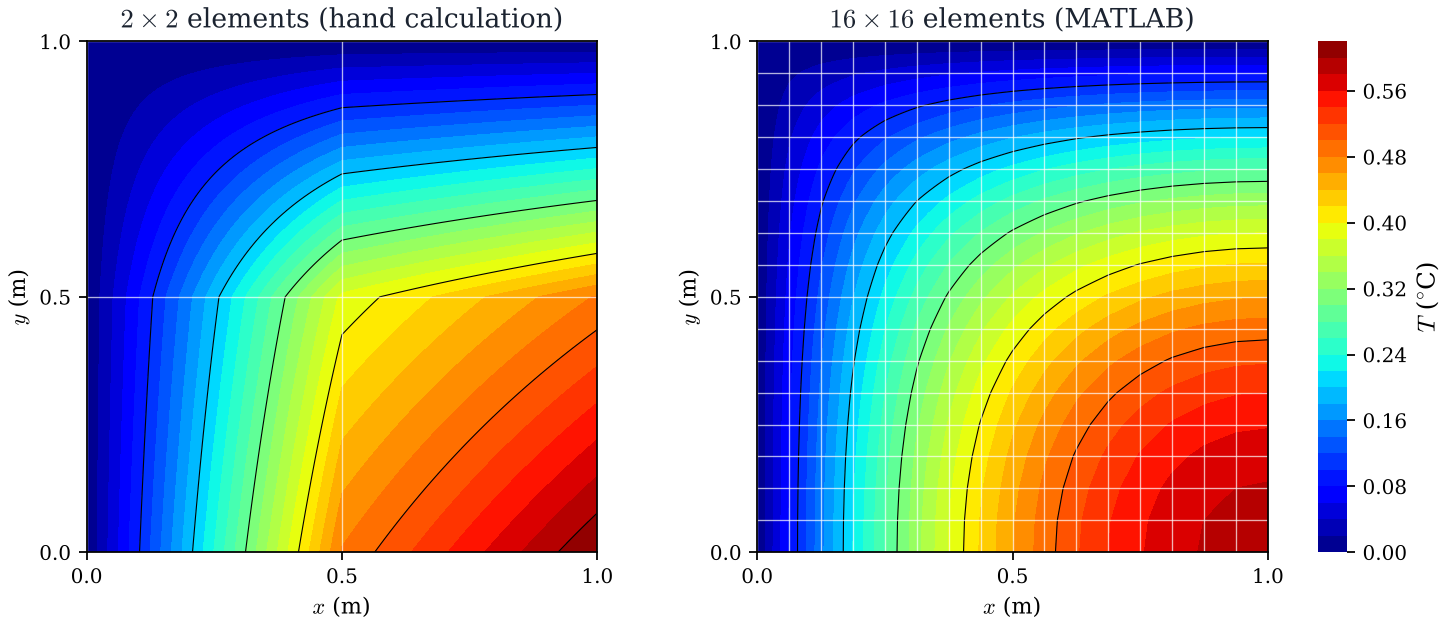
Temperature contours of the plate on the 2 by 2 mesh, faceted, and on a 16 by 16 mesh, smooth — Left: the 2 × 2 solution is faceted because each element is bilinear. Right: 16 × 16 is smooth and matches the text’s software value to the fourth decimal.Kiri: penyelesaian 2 × 2 berfaset kerana setiap element bilinear. Kanan: 16 × 16 licin dan sepadan dengan nilai perisian dalam teks hingga tempat perpuluhan keempat.

The habit of the courseTabiat kursus iniA convergence check is the same problem on a finer mesh; refine until the answer stops moving, and show the table. The error of bilinear elements falls about four times each time the mesh is halved.Semakan convergence ialah masalah yang sama pada mesh yang lebih halus; refine sehingga jawapan berhenti berubah, dan tunjukkan jadualnya. Ralat element bilinear jatuh kira-kira empat kali setiap kali mesh dibahagi dua.

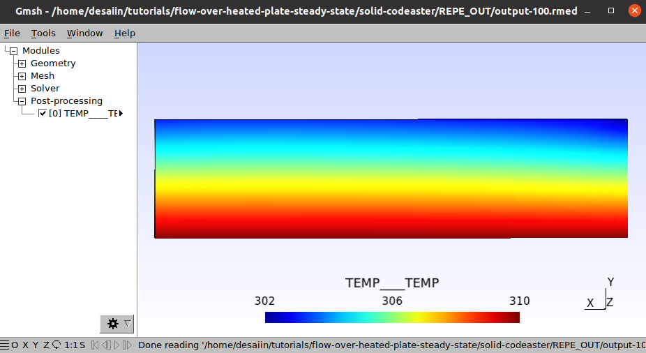
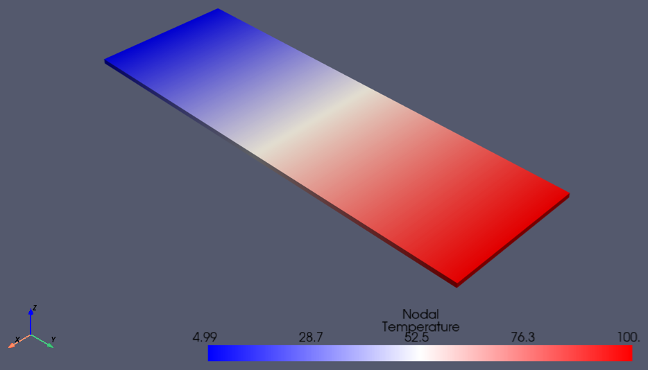
Temperature in a solid plate computed with Code_Aster, shown in Gmsh

ANSYS MAPDL nodal temperature in a plate held at 5 and 100 degrees on two opposite faces

Other codes, the same equations. Left: Code_Aster, preCICE tutorials “Flow over a heated plate, steady state”, LGPL-3.0. Right: ANSYS MAPDL, PyMAPDL documentation “Basic thermal analysis”, © ANSYS, Inc., MIT licence. With no source and two fixed faces the solution is linear and any mesh reproduces it exactly: a quick check of any new model.Kod lain, persamaan yang sama. Kiri: Code_Aster, tutorial preCICE “Flow over a heated plate, steady state”, LGPL-3.0. Kanan: ANSYS MAPDL, dokumentasi PyMAPDL “Basic thermal analysis”, © ANSYS, Inc., lesen MIT. Tanpa source dan dengan dua muka tetap, penyelesaiannya linear dan mana-mana mesh menghasilkannya dengan tepat: semakan pantas untuk mana-mana model baharu.

Key pointsPerkara utama

Post-process per element: locate, convert to local coordinates, interpolate with the nodal values in local order.Post-process setiap element: cari, tukar kepada koordinat local, interpolate dengan nilai node mengikut susunan local.
T(0.3, 0.2) = 0.266 °C; flux at the centroid of element 2 = (−70.7, +70.7) W m⁻².T(0.3, 0.2) = 0.266 °C; flux pada centroid element 2 = (−70.7, +70.7) W m⁻².
The 2 × 2 mesh is about 5% high; 16 × 16 matches software. Refine before you believe a number.Mesh 2 × 2 kira-kira 5% tinggi; 16 × 16 sepadan dengan perisian. Refine sebelum anda percaya sesuatu nombor.

Quick check · not gradedSemak cepat · tidak bergred

The point (0.8, 0.2) m in the text’s 2 × 2 mesh (a = b = 0.5 m) lies in element 2. Its local coordinates areTitik (0.8, 0.2) m dalam mesh 2 × 2 teks (a = b = 0.5 m) terletak dalam element 2. Koordinat local-nya ialah

Mark this section as readTanda seksyen ini sudah dibacaRead ✓ — untick to review againSudah dibaca ✓ — nyahtanda untuk ulang

6. The script, the assignment and what comes nextSkrip, tugasan dan apa yang seterusnya

≈ 5 min

The script is the pipeline in thirty lines. Read it against the seven steps and every block has a name.Skrip ini ialah pipeline dalam tiga puluh baris. Baca ia berpandukan tujuh langkah dan setiap blok ada namanya.

% Local conductance matrix (text §2.3.1)
a = L/Nx; b = H/Ny;
s1 = b*kx/(3*a) + a*ky/(3*b);
s2 = -b*kx/(3*a) + a*ky/(6*b);
s3 = -b*kx/(6*a) - a*ky/(6*b);
s4 = b*kx/(6*a) - a*ky/(3*b);
k = [s1 s2 s3 s4; s2 s1 s4 s3; s3 s4 s1 s2; s4 s3 s2 s1];
fQ = a*b*Q/4*[1; 1; 1; 1];        % heat generation
% Assembly by connectivity (conn(e,:) = global nodes of element e)
for e = 1:Ne,  c = conn(e,:);  K(c,c) = K(c,c) + k;  F(c) = F(c) + fQ;  end
% Essential conditions: known nodes removed, their columns moved to the right
free = setdiff(1:n, fixed);  T = zeros(n,1);  T(fixed) = Tbar;
T(free) = K(free,free) \ (F(free) - K(free,fixed)*T(fixed));
% Post-processing: element, local coordinates, interpolation
e = find_element(x, y);  xl = x - X(conn(e,1));  yl = y - Y(conn(e,1));
N = [(a-xl)*(b-yl), xl*(b-yl), xl*yl, yl*(a-xl)]/(a*b);  Tp = N*T(conn(e,:));

Lines 2–8: step 5, the element matrix and load from the closed-form s₁…s₄ of §2.Baris 2–8: langkah 5, matrix element dan load daripada s₁…s₄ closed-form dalam §2.
Line 10: step 6, assembly, one scatter-add per element.Baris 10: langkah 6, assembly, satu scatter-add setiap element.
Lines 12–13: step 6, the known temperatures moved to the right and struck; step 7, the backslash solve.Baris 12–13: langkah 6, temperature yang diketahui dipindahkan ke kanan dan dibuang; langkah 7, penyelesaian backslash.
Lines 15–16: §5, interpolation in local coordinates.Baris 15–16: §5, interpolation dalam koordinat local.

Try itCubaChange the mesh to 4 × 4 and compare T(1, 0) with the table of §5. Then set Q = 0 and T = 5 on the left and 100 on the right edge: every mesh must return a straight line.Tukar mesh kepada 4 × 4 dan bandingkan T(1, 0) dengan jadual §5. Kemudian tetapkan Q = 0 dan T = 5 di kiri dan 100 di tepi kanan: setiap mesh mesti memulangkan garis lurus.

Assignment 4 · what is askedTugasan 4 · apa yang diminta

Three identical 2 m × 3 m elements, T = 100 K on the left edge, zero flux elsewhere, a heat source on element 1.Tiga element 2 m × 3 m yang serupa, T = 100 K pada tepi kiri, flux sifar di tempat lain, satu heat source pada element 1.

(a) The local load vector {r¹} for the heat source Q = 20 W m⁻² on element 1 (unit thickness).(a) Load vector local {r¹} bagi heat source Q = 20 W m⁻² pada element 1 (ketebalan unit).
(b) The global [K] in terms of k, with k_x = k_y = k, using the connectivity table of Activity 3.(b) [K] global dalam sebutan k, dengan k_x = k_y = k, menggunakan connectivity table Aktiviti 3.
(c) With T₂ = T₆ = 150 K from the solution, interpolate T at (x, y) = (1.4, 2.2) m.(c) Dengan T₂ = T₆ = 150 K daripada penyelesaian, interpolate T pada (x, y) = (1.4, 2.2) m.

Show the connectivity table, s₁…s₄ with a = 2 m, b = 3 m, and the local coordinates used in (c). Marks are for the method; state the convention you use for the source (per unit area, unit thickness). Individual work.Tunjukkan connectivity table, s₁…s₄ dengan a = 2 m, b = 3 m, dan koordinat local yang digunakan dalam (c). Markah diberi untuk kaedah; nyatakan konvensyen yang anda guna untuk source (per unit luas, ketebalan unit). Kerja individu.

What comes nextApa yang seterusnya

Plane stress repeats every step of this part with two unknowns per node: [E] becomes 3 × 3, {∂} a 2 × 3 operator matrix, and [k] 8 × 8. Before that session, read text §3.1 and revise plane stress versus plane strain, Hooke’s law in 2D and the strain–displacement relations.Plane stress mengulang setiap langkah bahagian ini dengan dua unknown setiap node: [E] menjadi 3 × 3, {∂} matrix operator 2 × 3, dan [k] 8 × 8. Sebelum sesi itu, baca teks §3.1 dan ulang kaji plane stress berbanding plane strain, hukum Hooke dalam 2D dan hubungan strain–displacement.

Key pointsPerkara utama

Seven steps, thirty lines: element matrix, scatter-add assembly, strike the known nodes, backslash, interpolate in local coordinates.Tujuh langkah, tiga puluh baris: matrix element, assembly scatter-add, buang node yang diketahui, backslash, interpolate dalam koordinat local.
Assignment 4: {r¹}, [K] in terms of k, T at (1.4, 2.2) — method marks; show the bookkeeping.Tugasan 4: {r¹}, [K] dalam sebutan k, T pada (1.4, 2.2) — markah kaedah; tunjukkan rekod.

Quick check · not gradedSemak cepat · tidak bergred

With no heat source and two opposite edges held at fixed temperatures, a 1 × 1 mesh of one bilinear element givesTanpa heat source dan dua tepi bertentangan ditetapkan pada temperature tetap, mesh 1 × 1 dengan satu element bilinear memberi

Mark this section as readTanda seksyen ini sudah dibacaRead ✓ — untick to review againSudah dibaca ✓ — nyahtanda untuk ulang

SlidesSlides

What to doApa perlu dibuat Step through with ◀ ▶ (⏮ ⏭ for the first and last), the ← → keys, the mouse wheel or a swipe on the slide, or drag the bar under the slide to any page; the list below jumps to any slide. Download the PDF for printing and offline reading.Gerak dengan ◀ ▶ (⏮ ⏭ untuk slide pertama dan terakhir), kekunci ← →, roda tetikus atau leret pada slide, atau seret bar di bawah slide ke mana-mana halaman; senarai di bawah melompat ke mana-mana slide. Muat turun PDF untuk cetakan dan bacaan luar talian.

Counts toward progress:Dikira dalam kemajuan: each slide you open, once.setiap slide yang anda buka, sekali.

1 / 45

Loading slides…Memuatkan slides…

ExamplesContoh

What to doApa perlu dibuat Model answers in exam form, with suggested marks. Try each question on paper first, then compare step by step; tick it at the end when you have worked through it.Jawapan model dalam bentuk peperiksaan, dengan markah cadangan. Cuba setiap soalan di atas kertas dahulu, kemudian bandingkan langkah demi langkah; tandanya di hujung apabila anda sudah mengikutinya.

Counts toward progress:Dikira dalam kemajuan: examples ticked as worked through.contoh yang ditanda sudah diikuti.

How this topic is examinedBagaimana topik ini diuji

Model answers in the form the examiner expects: physical picture, plan, numbered steps with every substitution written out, checks, a boxed answer and an interpretation. The marks shown are a suggested scheme for a 20-mark question; the examiner’s own scheme may differ.Jawapan model dalam bentuk yang pemeriksa jangkakan: gambaran fizikal, pelan, langkah bernombor dengan setiap penggantian ditulis, semakan, jawapan berkotak dan tafsiran. Markah yang ditunjukkan ialah skema cadangan untuk soalan 20 markah; skema pemeriksa sendiri mungkin berbeza.

Question typeJenis soalan	Given and wantedDiberi dan dikehendaki	Plan and the usual trapPelan dan perangkap biasa
Shape functionsShape function	Node coordinates and the interpolation polynomial; wanted: N_i.Koordinat node dan polynomial interpolation; dikehendaki: N_i.	Nodal conditions, solve for a_i, collect the T_i. Trap: no check of N_i = 1 at node i and 0 at the others.Nodal condition, selesaikan a_i, kumpulkan T_i. Perangkap: tiada semakan N_i = 1 pada node i dan 0 pada node lain.
Temperature at a pointTemperature pada satu titik	Nodal temperatures; wanted: T(x, y), sometimes the flux.Nodal temperature; dikehendaki: T(x, y), kadang-kadang flux.	Find the element, use its local coordinates in N_i. Trap: global x, y in N_i.Cari element, guna koordinat local dalam N_i. Perangkap: x, y global dalam N_i.
Conductance matrixConductance matrix	a, b, k_x, k_y (and t); wanted: [k], often in terms of k.a, b, k_x, k_y (dan t); dikehendaki: [k], selalunya dalam sebutan k.	s₁ to s₄ and the pattern of (2.49). Trap: b/a and a/b swapped.s₁ hingga s₄ dan pola (2.49). Perangkap: b/a dan a/b tertukar.
Heat loadsLoad haba	Q or q_n on an element; wanted: {r}.Q atau q_n pada satu element; dikehendaki: {r}.	Equal shares. Trap: Q in W/m² against W/m³.Bahagian sama rata. Perangkap: Q dalam W/m² berbanding W/m³.
Assembly and solutionAssembly dan penyelesaian	Identical elements, prescribed temperatures, insulated edges; wanted: the free nodal temperatures.Element serupa, temperature ditetapkan, tepi insulated; dikehendaki: temperature node bebas.	K_ii is s₁ times the number of elements at node i; strike the fixed nodes; use symmetry.K_ii ialah s₁ kali bilangan element pada node i; buang node tetap; guna simetri.
ExplainTerangkan	Imposing T = T̄; insulated edges; why a row adds up to zero.Mengenakan T = T̄; tepi insulated; mengapa satu baris berjumlah sifar.	Claim, reason, consequence — three sentences, in that order.Dakwaan, sebab, akibat — tiga ayat, mengikut urutan itu.

Notation follows the companion: Q is the heat generated per unit volume (the text’s q_h), q_n the inward boundary flux (the text’s q_b), t the thickness.Notasi mengikut buku pendamping: Q ialah haba dijana per unit isi padu (q_h dalam teks), q_n boundary flux ke dalam (q_b dalam teks), t ketebalan.

Example 1 · Conductance matrix and nodal loads of a square elementContoh 1 · Conductance matrix dan nodal load bagi element segi empat sama

Exam typeJenis soalan [k] of a Q4 element, two entries by integration, the rest by pattern; {b} for a boundary flux, {q} for a sourceUnitsUnit W, m, KSourceSumber FEM by Hand, Examples 8.2 and 8.3 (textbook Exercises 2.1–2.3)20 marksmarkah

QuestionSoalanA square element of side 0.025 m and thickness 0.005 m has k = 450 W m⁻¹ K⁻¹. (a) Show the integration for k₁₂ and k₁₃ and complete [k] by the pattern of (2.49). (b) Determine the nodal loads for an inward heat flux of 10⁶ W m⁻² on its right side, 2–3, and (c) for an internal heat generation of 10⁷ W m⁻³. (d) In an examination plate of unit thickness, an element 2 m wide and 3 m high carries a heat source Q = 20 W m⁻²; determine its load vector.

The element of Example 1.Element bagi Contoh 1.

Physical picture.Gambaran fizikal. k_ij is the heat that must be supplied at node i when node j is held 1 K above the others, all at 0 K. In a square it is negative for i ≠ j, because a hotter node j pushes heat towards node i and the supply at i must take it away. For a square with k_x = k_y the matrix depends only on k and t, not on the side. The heat entering or generated is shared by the nodes in proportion to how much each shape function covers: every N_i integrates to ab/4 over the element, and along a side only its two nodes have non-zero shape functions, each taking half.k_ij ialah haba yang mesti dibekalkan pada node i apabila node j ditahan 1 K lebih tinggi daripada yang lain, semuanya pada 0 K. Dalam segi empat sama ia negatif untuk i ≠ j, kerana node j yang lebih panas menolak haba ke arah node i dan bekalan di i mesti membawanya pergi. Bagi segi empat sama dengan k_x = k_y, matrix itu bergantung pada k dan t sahaja, bukan pada sisi. Haba yang masuk atau dijana dikongsi oleh node mengikut kadar liputan setiap shape function: setiap N_i ber-integral kepada ab/4 di atas element, dan di sepanjang satu sisi hanya dua node-nya mempunyai shape function bukan sifar, setiap satu mengambil separuh.

Plan. Derivatives of N₁, N₂, N₃ → integrate k₁₂, k₁₃ → s₁ to s₄ → the pattern → row-sum check → (b) {b} on side 2–3 → (c) {q} → (d) the same with Q per unit area → totals as checks.

Step 1 DerivativesDerivative[2]

From (8.5), the shape functions of Part 1:Daripada (8.5), shape function Part 1:

Step 2 (a) Two entries by integration(a) Dua entri melalui integration[5]

Step 3 (a) Numbers(a) Nombor[3]

With a = b and k_x = k_y = 450, multiplied by t = 0.005 m:Dengan a = b dan k_x = k_y = 450, didarab dengan t = 0.005 m:

Step 4 (a) The matrix(a) Matrix[2]

Check. Every row: 1.5 − 0.375 − 0.75 − 0.375 = 0.

Answer. (a) [k] as above: s₁ = 1.5, s₂ = s₄ = −0.375, s₃ = −0.75 W K⁻¹.

Step 5 (b) Flux on side 2–3(b) Flux pada sisi 2–3[3]

On x = a: N₁ = N₄ = 0, N₂ = (b − y)/b, N₃ = y/b. Each integrates to b/2 along the side:Pada x = a: N₁ = N₄ = 0, N₂ = (b − y)/b, N₃ = y/b. Setiap satu ber-integral kepada b/2 di sepanjang sisi:

Check. Total 125 W = q_n t b = 10⁶(0.005)(0.025), the heat crossing the side.

Step 6 (c) Heat generation(c) Heat generation[3]

∫N_i dA = ab/4 for each node, so∫N_i dA = ab/4 bagi setiap node, jadi

Check. Total 31.25 W = Q t ab.

Step 7 (d) A source given per unit area(d) Source yang diberi per unit luas[2]

Q = 20 W m⁻² is heat per unit area of the plate and already contains the thickness, so it is not multiplied by t:Q = 20 W m⁻² ialah haba per unit luas plat dan sudah mengandungi ketebalan, jadi ia tidak didarab dengan t:

Answer. (b) 62.5 W at nodes 2 and 3. (c) 7.81 W at each node. (d) {r}¹ = {30, 30, 30, 30}ᵀ W.

Pitfall · W m⁻² or W m⁻³Perangkap · W m⁻² atau W m⁻³A source per unit volume (W m⁻³) is multiplied by t. A source per unit area of the plate (W m⁻²), as in part (d), already contains the thickness: do not multiply again.Source per unit isi padu (W m⁻³) didarab dengan t. Source per unit luas plat (W m⁻²), seperti dalam bahagian (d), sudah mengandungi ketebalan: jangan darab lagi.

InterpretationTafsiranThe diagonal pair (1–3) is coupled twice as strongly as each side pair, −0.75 against −0.375 W K⁻¹. For a side pair the two directions work against each other: in k₁₂ the k_x term is negative and the k_y term positive; for a diagonal pair both are negative. Doubling the side of the square leaves [k] unchanged: the longer conduction path and the wider section cancel. Equal shares are a property of uniform loads; whatever the distribution, the loads must add up to the total heat, and that check catches a forgotten thickness or a misplaced factor of 2.Pasangan pepenjuru (1–3) digandingkan dua kali lebih kuat daripada setiap pasangan sisi, −0.75 berbanding −0.375 W K⁻¹. Bagi pasangan sisi, dua arah itu bertentangan: dalam k₁₂ term k_x negatif dan term k_y positif; bagi pasangan pepenjuru kedua-duanya negatif. Menggandakan sisi segi empat sama tidak mengubah [k]: laluan conduction yang lebih panjang dan keratan yang lebih lebar saling membatalkan. Bahagian sama rata ialah sifat load seragam; apa jua taburannya, load mesti berjumlah kepada jumlah haba, dan semakan itu menangkap ketebalan yang terlupa atau faktor 2 yang tersalah letak.

Marking scheme (suggested)Skema pemarkahan (cadangan) · 20

What earns the marksApa yang diberi markah	MarksMarkah
Derivatives of the shape functionsDerivative shape function	2
k₁₂ and k₁₃ by integration, with the integrals evaluatedk₁₂ dan k₁₃ melalui integration, dengan integral dinilai	5
Numerical s₁…s₄ with ts₁…s₄ berangka dengan t	3
Matrix by the pattern, row-sum checkMatrix mengikut pola, semakan jumlah baris	2
{b}: half the flux × length × t at each of the two nodes, total check{b}: separuh flux × panjang × t pada setiap dua node, semakan jumlah	3
{q}: tQab/4 at each node, total check{q}: tQab/4 pada setiap node, semakan jumlah	3
Per-unit-area source not multiplied by tSource per unit luas tidak didarab dengan t	2
TotalJumlah	20

Mark this example as worked throughTanda contoh ini sudah diikutiWorked through ✓ — untick to revisitSudah diikuti ✓ — nyahtanda untuk ulang

Example 2 · Four elements with a prescribed temperature and an inward fluxContoh 2 · Empat element dengan temperature ditetapkan dan flux ke dalam

Exam typeJenis soalan assembly of a 2 × 2 mesh, essential and natural conditions, solution by symmetry, energy balanceUnitsUnit W, m, KSourceSumber FEM by Hand, Example 8.6 (textbook Exercise 2.4)20 marksmarkah

QuestionSoalanThe square plate of the figure, 0.05 m by 0.05 m and 0.005 m thick, is divided into four equal elements. Its top and bottom are insulated, its left side is held at 400 K, and its right side receives an inward heat flux of 10⁶ W m⁻². With k = 450 W m⁻¹ K⁻¹, determine the temperature at node 5.

The plate of Example 2 with the global node numbers.Plat bagi Contoh 2 dengan nombor node global.

Physical picture.Gambaran fizikal. The heat entering at the right side, 10⁶(0.005)(0.05) = 250 W, must all leave through the left side; with the top and bottom insulated it flows straight across, so T depends on x only. With no source the gradient is constant, q_n/k = 2222 K m⁻¹, so expect T = 400 + 2222x: 455.6 K at the middle column and 511.1 K at the right side. A bilinear element contains this linear field, so the finite element solution should reproduce it.Haba yang masuk pada sisi kanan, 10⁶(0.005)(0.05) = 250 W, mesti semuanya keluar melalui sisi kiri; dengan atas dan bawah insulated ia mengalir terus melintang, jadi T bergantung pada x sahaja. Tanpa source, gradient-nya malar, q_n/k = 2222 K m⁻¹, jadi jangkakan T = 400 + 2222x: 455.6 K pada lajur tengah dan 511.1 K pada sisi kanan. Element bilinear mengandungi field linear ini, jadi penyelesaian finite element sepatutnya menghasilkannya semula.

Plan. [k] of Example 1 → assemble 9 × 9 → flux loads at nodes 3, 6, 9 → strike nodes 1, 4, 7 → solve by columns → check a full row → energy balance.

Step 1 Element matrices and assemblyMatrix element dan assembly[5]

The four elements are identical to that of Example 1. With element 1 on nodes 1, 2, 5, 4 (local 1, 2, 3, 4), element 2 on 2, 3, 6, 5, element 3 on 4, 5, 8, 7 and element 4 on 5, 6, 9, 8:Keempat-empat element serupa dengan element Contoh 1. Dengan element 1 pada node 1, 2, 5, 4 (local 1, 2, 3, 4), element 2 pada 2, 3, 6, 5, element 3 pada 4, 5, 8, 7 dan element 4 pada 5, 6, 9, 8:

Corner nodes have ts₁ = 1.5, side nodes 2ts₁ = 3, the centre 4ts₁ = 6 W K⁻¹.Node bucu mempunyai ts₁ = 1.5, node sisi 2ts₁ = 3, pusat 4ts₁ = 6 W K⁻¹.

Step 2 LoadsLoad[3]

The flux enters through sides 3–6 and 6–9, each giving 62.5 W to each of its nodes (Example 1):Flux masuk melalui sisi 3–6 dan 6–9, setiap satu memberi 62.5 W kepada setiap node-nya (Contoh 1):

Step 3 Boundary conditionsBoundary condition[3]

T₁ = T₄ = T₇ = 400 K: strike rows and columns 1, 4, 7 and subtract K_i1(400) + K_i4(400) + K_i7(400) from the right-hand side. Six unknowns remain.T₁ = T₄ = T₇ = 400 K: buang baris dan lajur 1, 4, 7 dan tolak K_i1(400) + K_i4(400) + K_i7(400) daripada sebelah kanan. Enam unknown tinggal.

Step 4 Solution by columnsPenyelesaian mengikut lajur[5]

Since T does not vary with y, the middle column shares one value and the right column another. Adding the three equations of the middle column (rows 2, 5, 8) and the three of the right column (rows 3, 6, 9):Oleh kerana T tidak berubah dengan y, lajur tengah berkongsi satu nilai dan lajur kanan satu nilai lain. Menambah tiga persamaan lajur tengah (baris 2, 5, 8) dan tiga persamaan lajur kanan (baris 3, 6, 9):

Check.

Answer. T₅ = 455.6 K (and T₂ = T₈ = 455.6, T₃ = T₆ = T₉ = 511.1 K).

Step 5 Energy balanceEnergy balance[4]

InterpretationTafsiranThe finite element temperatures equal the exact 400 + q_nx/k at every node, as expected: the exact field is linear, and a bilinear element represents a linear field exactly. Two features of the data make the column shortcut valid, the insulated top and bottom and the uniform conditions on the left and right; with a flux on part of a side only, or a hole, T would vary with y and the six equations would have to be solved together. Doubling the thickness doubles both [K] and {R} and leaves the temperatures unchanged.

Temperature finite element sama dengan 400 + q_nx/k yang tepat pada setiap node, seperti dijangka: field tepat adalah linear, dan element bilinear mewakili field linear dengan tepat. Dua ciri data menjadikan jalan pintas lajur itu sah, iaitu atas dan bawah yang insulated dan keadaan seragam di kiri dan kanan; dengan flux pada sebahagian sisi sahaja, atau satu lubang, T akan berubah dengan y dan enam persamaan itu perlu diselesaikan bersama. Menggandakan ketebalan menggandakan [K] dan {R} dan tidak mengubah temperature.

Marking scheme (suggested)Skema pemarkahan (cadangan) · 20

What earns the marksApa yang diberi markah	MarksMarkah
[K] assembled with the right multiplicities (1.5, 3, 6 on the diagonal)[K] di-assemble dengan gandaan yang betul (1.5, 3, 6 pada pepenjuru)	5
Flux loads at nodes 3, 6, 9Load flux pada node 3, 6, 9	3
Rows and columns 1, 4, 7 struck, 400 K moved to the rightBaris dan lajur 1, 4, 7 dibuang, 400 K dipindahkan ke kanan	3
Column equations and T₅; a full-row checkPersamaan lajur dan T₅; semakan satu baris penuh	5
Struck rows give 250 W out = 250 W inBaris yang dibuang memberi 250 W keluar = 250 W masuk	4
TotalJumlah	20

Mark this example as worked throughTanda contoh ini sudah diikutiWorked through ✓ — untick to revisitSudah diikuti ✓ — nyahtanda untuk ulang

Example 3 · Plate with a heat source: the textbook’s worked exampleContoh 3 · Plat dengan heat source: contoh bekerja dalam teks

Exam typeJenis soalan 2 × 2 mesh, assembly, symmetry, energy balance, accuracyUnitsUnit W, m, °CSourceSumber FEM by Hand, Example 8.7 (textbook §2.3)20 marksmarkah

QuestionSoalanThe square plate of the figure, 1 m by 1 m and of unit thickness, generates Q = 600 W m⁻³ and has k = 300 W m⁻¹ °C⁻¹. Its left and top edges are held at 0 °C; its bottom and right edges are insulated. With four equal Q4 elements, (a) form [k] and {r} of an element, (b) assemble, apply the boundary conditions and solve, and (c) check the energy balance and compare with the exact solution.

The plate (textbook Figs. 2.5 and 2.6).Plat (teks Rajah 2.5 dan 2.6).

The mesh with its global node numbers.Mesh dengan nombor node global-nya.

Physical picture.Gambaran fizikal. The heat generated everywhere flows to the cold left and top edges, so the hottest point is the corner farthest from both, node 3 at (1, 0). The problem is symmetric about the diagonal through (0, 1) and (1, 0), so T₂ = T₆. The insulated edges are lines of symmetry: the plate is one quarter of a 2 m square with all edges at 0 °C, whose centre temperature is 0.07367 Q(2)²/k = 0.589 °C.Haba yang dijana di mana-mana mengalir ke tepi kiri dan atas yang sejuk, jadi titik paling panas ialah bucu paling jauh daripada kedua-duanya, node 3 pada (1, 0). Masalah ini simetri tentang pepenjuru melalui (0, 1) dan (1, 0), jadi T₂ = T₆. Tepi insulated ialah garis simetri: plat ini ialah satu perempat daripada segi empat sama 2 m dengan semua tepi pada 0 °C, yang temperature pusatnya 0.07367 Q(2)²/k = 0.589 °C.

Plan. s₁ to s₄, Qab/4 → assemble 9 × 9 → strike nodes 1, 4, 7, 8, 9 → T₆ = T₂ → 3 × 3 → heat flows → exact solution and convergence.

Step 1 (a) Element matrices(a) Matrix element[3]

Step 2 (b) Assembly(b) Assembly[4]

Corner nodes belong to one element, side nodes to two and node 5 to four:Node bucu dimiliki satu element, node sisi dua dan node 5 empat:

The complete 9 × 9 is (2.53) of the textbook; its rows for the free nodes, after striking T₁ = T₄ = T₇ = T₈ = T₉ = 0 (nothing moves to the right, since the prescribed temperatures are zero):9 × 9 yang lengkap ialah (2.53) dalam teks; barisnya bagi node bebas, selepas membuang T₁ = T₄ = T₇ = T₈ = T₉ = 0 (tiada yang berpindah ke kanan, kerana temperature yang ditetapkan ialah sifar):

Step 3 (b) Solution with T₆ = T₂(b) Penyelesaian dengan T₆ = T₂[5]

Row 6 then repeats row 2, and the other three rows becomeBaris 6 kemudian mengulang baris 2, dan tiga baris yang lain menjadi

The second gives T₃ = 0.1875 + 0.5T₂ + 0.5T₅. Substituting into the first and the third:Yang kedua memberi T₃ = 0.1875 + 0.5T₂ + 0.5T₅. Menggantikan ke dalam yang pertama dan ketiga:

Check. Row 1 of the reduced system: 400(0.4821) − 50(0.6214) − 100(0.3857) − 100(0.4821) = 75.0 ✓

Answer. (b) T₂ = T₆ = 0.482, T₃ = 0.621, T₅ = 0.386 °C, the textbook’s (2.55).

Step 4 (c) Energy balance(c) Energy balance[4]

All the heat generated, Q × area = 600 W, leaves through the cold edges.Semua haba yang dijana, Q × luas = 600 W, keluar melalui tepi sejuk.

Step 5 (c) Comparison with the exact solution(c) Perbandingan dengan penyelesaian tepat[4]

At nodes 2, 3 and 5 the 2 × 2 mesh is 5.1%, 5.4% and 6.5% high. For the corner temperature:Pada node 2, 3 dan 5, mesh 2 × 2 adalah 5.1%, 5.4% dan 6.5% tinggi. Bagi temperature bucu:

meshmesh	1 × 1	2 × 2	4 × 4	8 × 8	16 × 16	exacttepat
T₃ (°C)	0.7500	0.6214	0.5968	0.5912	0.5898	0.5894
errorralat	+27.3%	+5.4%	+1.26%	+0.31%	+0.08%	–

Answer. (c) Energy balance 600 W in and out; the 2 × 2 mesh is 5–7% high at its nodes, and the error falls about four times each time the mesh is halved.

InterpretationTafsiranThe error falls as h², the rate of bilinear elements for a smooth field, about four times for each halving of the mesh. Finite element temperatures are not bounds: the 2 × 2 Q4 mesh is above the exact values, while the textbook’s two eight-node elements give 0.4448 and 0.5836 °C, below them. The nodal temperatures are not exact here, as they were in Example 2, because the exact field is curved in both directions. Node 5 shows the averaging property of square meshes: 800T₅ = 100(T₁ + … + T₉ without T₅) + 150, the mean of its eight neighbours plus the effect of the source.Ralat jatuh sebagai h², kadar element bilinear bagi field yang licin, kira-kira empat kali bagi setiap pembahagian dua mesh. Temperature finite element bukan sempadan: mesh Q4 2 × 2 berada di atas nilai tepat, manakala dua element lapan node dalam teks memberi 0.4448 dan 0.5836 °C, di bawahnya. Nodal temperature tidak tepat di sini, tidak seperti dalam Contoh 2, kerana field tepat melengkung dalam kedua-dua arah. Node 5 menunjukkan sifat purata mesh segi empat sama: 800T₅ = 100(T₁ + … + T₉ tanpa T₅) + 150, min lapan jirannya ditambah kesan source.

Marking scheme (suggested)Skema pemarkahan (cadangan) · 20

What earns the marksApa yang diberi markah	MarksMarkah
s₁…s₄ and Qab/4s₁…s₄ dan Qab/4	3
Diagonal multiplicities and the reduced 4 × 4Gandaan pepenjuru dan 4 × 4 terkurang	4
Symmetry used, 3 × 3 solved, a row checkSimetri digunakan, 3 × 3 diselesaikan, semakan satu baris	5
Heat flows at the cold nodes summing to −600 WAliran haba pada node sejuk berjumlah −600 W	4
Comparison with the exact values and the h² ratePerbandingan dengan nilai tepat dan kadar h²	4
TotalJumlah	20

Mark this example as worked throughTanda contoh ini sudah diikutiWorked through ✓ — untick to revisitSudah diikuti ✓ — nyahtanda untuk ulang

ExercisesLatihan

What to doApa perlu dibuat Start the timer. For each question choose Sure or Not sure first, then answer. The summary at the end compares your confidence with your results.Mulakan timer. Untuk setiap soalan pilih Yakin atau Tak pasti dahulu, kemudian jawab. Ringkasan di hujung membandingkan keyakinan anda dengan keputusan.

Counts toward progress:Dikira dalam kemajuan: questions answered (B: checked, or solution viewed).soalan yang dijawab (B: disemak, atau penyelesaian dilihat).

0:00targetsasaran 35 min · 1.5 min/markmarkah

A Concept questionsSoalan konsep · 6 × 1 markmarkah

Click one option. One try: the right answer is marked ✓ and explained.Klik satu pilihan. Satu cubaan: jawapan betul ditanda ✓ dan diterangkan.

A1 · 1 markmarkah
Integration by parts is applied to the weighted residual mainly in order toIntegration by parts digunakan pada weighted residual terutamanya untuk

Before you answer:Sebelum menjawab:

A2 · 1 markmarkah
For the text’s plate (top and left edges at 0 °C, right and bottom insulated), the boundary vector {b} of every element isBagi plat dalam teks (tepi atas dan kiri pada 0 °C, kanan dan bawah insulated), boundary vector {b} setiap element ialah

Before you answer:Sebelum menjawab:

A3 · 1 markmarkah
For an element with a = 2 m, b = 1 m and k_x = k_y = k, the entry s₂ isBagi element dengan a = 2 m, b = 1 m dan k_x = k_y = k, entri s₂ ialah

Before you answer:Sebelum menjawab:

A4 · 1 markmarkah
In the 2 × 2 mesh the diagonal entry K₅₅ of the centre node equalsDalam mesh 2 × 2, entri pepenjuru K₅₅ bagi node pusat bersamaan

Before you answer:Sebelum menjawab:

A5 · 1 markmarkah
The struck rows of a node with a prescribed temperature are useful because they giveBaris yang dibuang bagi node dengan temperature yang ditetapkan berguna kerana ia memberi

Before you answer:Sebelum menjawab:

A6 · 1 markmarkah
Refining the text’s mesh from 2 × 2 to 4 × 4 changes T(1, 0) from 0.6214 to 0.5968 °C (exact 0.5894). Halving the mesh again should leave an error of aboutMenghalusi mesh teks dari 2 × 2 kepada 4 × 4 mengubah T(1, 0) dari 0.6214 kepada 0.5968 °C (tepat 0.5894). Membahagi dua mesh sekali lagi sepatutnya meninggalkan ralat kira-kira

Before you answer:Sebelum menjawab:

B Calculation, new numbers each timePengiraan, nombor baharu setiap kali · 16 marksmarkah

Type your numbers and press Check; each field is marked ✓ or ✗. Retry as often as you like, open hints one at a time, or show the solution. New numbers gives a fresh version.Taip nombor anda dan tekan Semak; setiap ruang ditanda ✓ atau ✗. Cuba semula seberapa kerap, buka petunjuk satu demi satu, atau tunjuk penyelesaian. Nombor baharu memberi versi baharu.

B1 · The four values of the conductance matrixEmpat nilai conductance matrix

4 marksmarkah

B2 · Source and edge-flux loadsLoad source dan flux tepi

3 marksmarkah

B3 · Assembly entries of a two-element stripEntri assembly bagi jalur dua element

4 marksmarkah

B4 · Temperature and flux at a point of the solved meshTemperature dan flux pada satu titik mesh yang diselesaikan

5 marksmarkah

C Find the slipCari kesilapan · 2 marksmarkah

Click the line that contains the error. One try.Klik baris yang mengandungi kesilapan. Satu cubaan.

C1 · 2 marksmarkah
A student interpolates T at (0.8, 0.2) m in the text’s solved 2 × 2 mesh (a = b = 0.5 m; T₂ = 0.482, T₃ = 0.621, T₅ = 0.386, T₆ = 0.482 °C). One line contains the slip. Which one?Seorang pelajar interpolate T pada (0.8, 0.2) m dalam mesh 2 × 2 teks yang telah diselesaikan (a = b = 0.5 m; T₂ = 0.482, T₃ = 0.621, T₅ = 0.386, T₆ = 0.482 °C). Satu baris mengandungi kesilapan. Yang mana?

Before you answer:Sebelum menjawab:

∑ SummaryRingkasan

ExplorerExplorer

What to doApa perlu dibuat Work in the Heat Conduction Explorer (on a phone, open it in its own tab). Do the 4 tasks on the right; answers to the Explorer’s own questions are under “Check answer” inside it. Python code for assignments and projects, and a panel that runs short scripts in the browser, are at the bottom of this tab.Bekerja dalam Heat Conduction Explorer (di telefon, buka dalam tab sendiri). Buat 4 tugasan di sebelah kanan; jawapan kepada soalan Explorer ada di bawah “Check answer” di dalamnya. Kod Python untuk assignment dan projek, dan panel untuk menjalankan skrip pendek dalam browser, ada di bahagian bawah tab ini.

Counts toward progress:Dikira dalam kemajuan: tasks done.tugasan yang selesai.

⤓ Python codeKod Python

Small screen? Skrin kecil? Open the Explorer in its own tabBuka Explorer dalam tab sendiri. Tasks done there are recorded here when you come back.Tugasan yang selesai di situ direkod di sini apabila anda kembali.

TasksTugasan · Heat Conduction Explorer

Each task ticks itself when the Explorer sees it done. Tick by hand only if it does not.Setiap tugasan ditanda sendiri apabila Explorer melihatnya selesai. Tanda sendiri hanya jika ia tidak ditanda.

1Keep the text’s example on the 2 × 2 mesh. Read T at the bottom-right corner and at the middle of the bottom edge; tap the plate to probe.Kekalkan contoh teks pada mesh 2 × 2. Baca T pada bucu kanan bawah dan di tengah tepi bawah; ketik plat untuk probe.

✓

Ticks itself: Ditanda sendiri: detected on the first probe with the text’s settings on 2 × 2dikesan pada probe pertama dengan tetapan teks pada 2 × 2 ·

2Run the mesh study. From which mesh does the maximum temperature change by less than 1%? Which value would you report?Jalankan kajian mesh. Dari mesh manakah temperature maksimum berubah kurang daripada 1%? Nilai mana yang akan anda laporkan?

✓

Ticks itself: Ditanda sendiri: detected when the mesh study runs with the text’s settingsdikesan apabila kajian mesh dijalankan dengan tetapan teks ·

3Set the right edge to 0 °C as well. Where is the hottest point now, and why there?Tetapkan tepi kanan kepada 0 °C juga. Di mana titik paling panas sekarang, dan mengapa di situ?

✓

Ticks itself: Ditanda sendiri: detected when three edges are at the same temperature and the bottom is insulateddikesan apabila tiga tepi berada pada temperature yang sama dan bawah insulated ·

4Make all four edges insulated. What does the Explorer report, and what does it mean physically?Jadikan keempat-empat tepi insulated. Apa yang dilaporkan oleh Explorer, dan apa maksudnya secara fizikal?

✓

Ticks itself: Ditanda sendiri: detected when all four edges are insulateddikesan apabila keempat-empat tepi insulated ·

Python code for assignments and projectsKod Python untuk assignment dan projek

The same steps and notation as the notes, written out in plain Python. Use it to check every matrix and number of a hand calculation, and to run what is impractical by hand: mesh studies, contour plots, your own geometry and loads.Langkah dan notasi yang sama seperti nota, ditulis dalam Python biasa. Guna untuk menyemak setiap matrix dan nombor dalam pengiraan tangan, dan untuk menjalankan apa yang tidak praktikal dibuat dengan tangan: kajian mesh, contour plot, geometri dan beban anda sendiri.

Unzip, then install Python 3.8 or newer and run pip install numpy matplotlib (matplotlib only for the plots).Unzip, kemudian pasang Python 3.8 atau lebih baharu dan jalankan pip install numpy matplotlib (matplotlib hanya untuk plot).
Run python fe_heat_q4.py. It reproduces the course example; README.txt lists the output you should see.Jalankan python fe_heat_q4.py. Ia menghasilkan semula contoh kursus; README.txt menyenaraikan output yang sepatutnya keluar.
Read the docstring at the top of the file for the notation, numbering and units, and how to call it for your own problem.Baca docstring di bahagian atas fail untuk notasi, penomboran dan unit, dan cara memanggilnya untuk masalah anda sendiri.

A hand calculation is still a hand calculation: in a test or an assignment that asks for the steps, show them yourself.Pengiraan tangan tetap pengiraan tangan: dalam ujian atau assignment yang meminta langkah, tunjukkan sendiri.

Show the codeTunjuk kod · fe_heat_q4.py · 268 linesbaris

"""
SEAA 4243 Finite Element Method - steady 2D heat conduction with 4-node elements
================================================================================

Companion code for the Heat Conduction Explorer (2D Heat Transfer, Part 2).
It follows the seven steps of the course, in the text's notation
(Mohd Yassin et al., MSNM 2020, Chapter 2):

    1-2  mesh of a rectangular plate, L x H, Nx x Ny four-node elements
    5    element matrix [k] from the closed-form s1...s4         text (2.49)
         source loads {q} = t Q ab/4 at each node                text (2.39)
         edge-flux loads {b} = t q_n l/2 at each edge node        text (2.40)
    6    assembly by the connectivity table (scatter-add),
         known temperatures by row-column elimination
    7    solve; heat flows at the fixed nodes (energy balance);
         temperature and heat flux at any point

Mesh and numbering
    Nodes are numbered left to right, then bottom to top, starting at 1 in
    the printout (the text's 2 x 2 mesh: nodes 1-3 along the bottom, 7-9 along
    the top). Element e has local nodes 1-4 anticlockwise from its bottom-left
    corner, e.g. element 1 of the 2 x 2 mesh = global nodes [1 2 5 4].

Units
    Any consistent set; the examples use m, W and degC (or K).
    Q is heat generated per unit VOLUME (W/m3) and is multiplied by t.
    A source given per unit AREA of the plate (W/m2) already contains the
    thickness: use t = 1 and Q = that value.
    q_n is the INWARD boundary flux (W/m2); an insulated edge has q_n = 0.

Run
    python fe_heat_q4.py
        reproduces the text's worked example (Sec. 2.3), its energy balance
        and mesh study, and the 2 x 2 plate with an inward flux; saves a
        contour plot if matplotlib is installed.

Use for your own problem: edit the block at the bottom, or
    from fe_heat_q4 import solve_plate, temperature_at
    res = solve_plate(L=4, H=2, Nx=4, Ny=2, kx=10, ky=10,
                      edges={"left": ("T", 50), "right": ("flux", 200),
                             "top": ("insulated",), "bottom": ("insulated",)},
                      Q=lambda xc, yc: 100 if xc < 1 else 0)  # source in the first column only
    print(res["K"])                     # compare with your hand assembly
    print(temperature_at(res, 1.4, 0.7))

A hand calculation is still a hand calculation: use this script to check your
matrices and numbers, and show the steps yourself.

Requires Python 3.8+ and numpy; matplotlib only for the plot.
Course SEAA 4243, Faculty of Civil Engineering, Universiti Teknologi Malaysia.
Code: MIT licence.
"""
import numpy as np


# ---------------------------------------------------------------------------
# Step 5: element matrix and loads
# ---------------------------------------------------------------------------
def s_values(a, b, kx, ky):
    """The four distinct entries of [k] for an a x b rectangle, text (2.49)."""
    s1 = b * kx / (3 * a) + a * ky / (3 * b)
    s2 = -b * kx / (3 * a) + a * ky / (6 * b)
    s3 = -b * kx / (6 * a) - a * ky / (6 * b)
    s4 = b * kx / (6 * a) - a * ky / (3 * b)
    return s1, s2, s3, s4


def element_matrix(a, b, kx, ky, t=1.0):
    """Conductance matrix [k] (4 x 4, W/K). Every row adds up to zero."""
    s1, s2, s3, s4 = s_values(a, b, kx, ky)
    return t * np.array([[s1, s2, s3, s4],
                         [s2, s1, s4, s3],
                         [s3, s4, s1, s2],
                         [s4, s3, s2, s1]])


# ---------------------------------------------------------------------------
# Steps 1-2: mesh
# ---------------------------------------------------------------------------
def mesh(L, H, Nx, Ny):
    """Node coordinates (n x 2) and connectivity (ne x 4, 0-based) of a structured mesh."""
    a, b = L / Nx, H / Ny
    nodes = np.array([(i * a, j * b) for j in range(Ny + 1) for i in range(Nx + 1)], dtype=float)
    conn = []
    for j in range(Ny):
        for i in range(Nx):
            n1 = j * (Nx + 1) + i
            conn.append([n1, n1 + 1, n1 + Nx + 2, n1 + Nx + 1])
    return a, b, nodes, np.array(conn, dtype=int)


def edge_nodes(nodes, L, H, edge, tol=1e-9):
    """Indices of the nodes on one edge of the plate, ordered along it."""
    x, y = nodes[:, 0], nodes[:, 1]
    if edge == "bottom":
        idx = np.where(abs(y) < tol)[0]; key = x
    elif edge == "top":
        idx = np.where(abs(y - H) < tol)[0]; key = x
    elif edge == "left":
        idx = np.where(abs(x) < tol)[0]; key = y
    elif edge == "right":
        idx = np.where(abs(x - L) < tol)[0]; key = y
    else:
        raise ValueError("edge must be bottom, right, top or left")
    return idx[np.argsort(key[idx])]


# ---------------------------------------------------------------------------
# Steps 5-7: assemble, impose, solve, post-process
# ---------------------------------------------------------------------------
def solve_plate(L, H, Nx, Ny, kx, ky=None, edges=None, Q=0.0, t=1.0):
    """Solve a rectangular plate.

    edges: dict with keys "bottom", "right", "top", "left"; each value is
           ("T", value)  prescribed temperature (essential)
           ("flux", qn)  inward heat flux, W/m2 (natural)
           ("insulated",) zero flux (natural; nothing to do)
           A corner shared by two prescribed edges takes the value of the
           first in the order top, left, right, bottom.
    Q:     heat generated per unit volume, a number or a function Q(xc, yc)
           of the element centroid (for a source on some elements only).
    Returns a dict with the mesh, [K], {R}, the temperatures and the heat
    flows at the fixed nodes.
    """
    ky = kx if ky is None else ky
    edges = edges or {}
    a, b, nodes, conn = mesh(L, H, Nx, Ny)
    n = len(nodes)
    K = np.zeros((n, n))
    R = np.zeros(n)
    k = element_matrix(a, b, kx, ky, t)
    generated = 0.0
    for e, c in enumerate(conn):
        K[np.ix_(c, c)] += k                                   # scatter-add
        xc, yc = nodes[c].mean(axis=0)
        Qe = Q(xc, yc) if callable(Q) else Q
        R[c] += t * Qe * a * b / 4                             # {q}: equal shares
        generated += t * Qe * a * b
    flux_in = 0.0
    for name, bc in edges.items():
        if bc[0] == "flux":
            ids = edge_nodes(nodes, L, H, name)
            h = b if name in ("left", "right") else a
            for i0, i1 in zip(ids[:-1], ids[1:]):
                R[i0] += t * bc[1] * h / 2                     # {b}: half to each node of the side
                R[i1] += t * bc[1] * h / 2
                flux_in += t * bc[1] * h
    fixed = {}
    for name in ("top", "left", "right", "bottom"):
        bc = edges.get(name, ("insulated",))
        if bc[0] == "T":
            for i in edge_nodes(nodes, L, H, name):
                fixed.setdefault(int(i), float(bc[1]))
    if not fixed:
        raise ValueError("No edge has a prescribed temperature: [K] is singular "
                         "(the temperature level is undetermined).")
    known = np.array(sorted(fixed))
    Tbar = np.array([fixed[i] for i in known])
    free = np.setdiff1d(np.arange(n), known)
    T = np.zeros(n)
    T[known] = Tbar
    # row-column elimination: move K(:, known) * Tbar to the right, keep the free rows
    rhs = R[free] - K[np.ix_(free, known)] @ Tbar
    T[free] = np.linalg.solve(K[np.ix_(free, free)], rhs)
    heat = K[known] @ T - R[known]          # struck rows: heat supplied (+) or removed (-) there
    return dict(L=L, H=H, Nx=Nx, Ny=Ny, a=a, b=b, kx=kx, ky=ky, t=t, nodes=nodes, conn=conn,
                K=K, R=R, T=T, known=known, free=free, heat=heat,
                generated=generated, flux_in=flux_in)


def locate(res, x, y):
    """Element containing the global point (x, y), and the local coordinates there."""
    a, b = res["a"], res["b"]
    i = min(res["Nx"] - 1, max(0, int(np.floor(x / a + 1e-12))))
    j = min(res["Ny"] - 1, max(0, int(np.floor(y / b + 1e-12))))
    e = j * res["Nx"] + i
    x1, y1 = res["nodes"][res["conn"][e][0]]
    return e, x - x1, y - y1


def temperature_at(res, x, y):
    """T and the heat flux (qx, qy) at a global point, from the element that contains it."""
    a, b = res["a"], res["b"]
    e, xl, yl = locate(res, x, y)
    Te = res["T"][res["conn"][e]]                       # nodal values in LOCAL order
    N = np.array([(a - xl) * (b - yl), xl * (b - yl), xl * yl, yl * (a - xl)]) / (a * b)
    dN = np.array([[-(b - yl), (b - yl), yl, -yl],
                   [-(a - xl), -xl, xl, (a - xl)]]) / (a * b)
    g = dN @ Te
    return dict(element=e + 1, local=(xl, yl), N=N, T=float(N @ Te),
                qx=float(-res["kx"] * g[0]), qy=float(-res["ky"] * g[1]))


def print_matrix(M, scale=1.0, name="[K]"):
    with np.printoptions(precision=3, suppress=True, linewidth=160):
        print(f"{name}" + (f" / {scale:g}" if scale != 1 else "") + " =")
        print(M / scale)


def plot_temperature(res, filename="temperature.png"):
    try:
        import matplotlib.pyplot as plt
    except ImportError:
        print("matplotlib is not installed: skipping the plot")
        return None
    xs = np.linspace(0, res["L"], 121)
    ys = np.linspace(0, res["H"], max(31, int(121 * res["H"] / res["L"])))
    X, Y = np.meshgrid(xs, ys)
    Z = np.vectorize(lambda x, y: temperature_at(res, x, y)["T"])(X, Y)
    fig, ax = plt.subplots(figsize=(6, 6 * res["H"] / res["L"] + 0.6))
    cf = ax.contourf(X, Y, Z, levels=21, cmap="jet")
    ax.contour(X, Y, Z, levels=10, colors="k", linewidths=0.5)
    for c in res["conn"]:
        p = res["nodes"][list(c) + [c[0]]]
        ax.plot(p[:, 0], p[:, 1], color="w", lw=0.8)
    ax.set_aspect("equal"); ax.set_xlabel("x (m)"); ax.set_ylabel("y (m)")
    fig.colorbar(cf, ax=ax, label="T")
    fig.savefig(filename, dpi=150, bbox_inches="tight")
    plt.close(fig)
    print("saved", filename)
    return filename


# ---------------------------------------------------------------------------
# Course examples
# ---------------------------------------------------------------------------
if __name__ == "__main__":
    # The text's worked example (Sec. 2.3): 1 m square, Q = 600 W/m3, k = 300,
    # top and left edges at 0 degC, right and bottom insulated, unit thickness.
    book = {"top": ("T", 0.0), "left": ("T", 0.0), "right": ("insulated",), "bottom": ("insulated",)}
    res = solve_plate(1, 1, 2, 2, 300, edges=book, Q=600)
    print("Text Sec. 2.3, 2 x 2 mesh")
    print("  element s1..s4 =", np.round(s_values(0.5, 0.5, 300, 300), 3), " (expected 200 -50 -100 -50)")
    print_matrix(res["K"], name="  [K]")
    print("  {R} =", res["R"])
    T = res["T"]
    print(f"  T2 = T6 = {T[1]:.4f}, T3 = {T[2]:.4f}, T5 = {T[4]:.4f} degC  (text (2.55): 0.4821, 0.6214, 0.3857)")
    print("  heat at fixed nodes", [int(i) + 1 for i in res["known"]], "=", np.round(res["heat"], 2), "W")
    print(f"  energy balance: generated {res['generated']:.1f} W, removed {-res['heat'].sum():.1f} W")
    p = temperature_at(res, 0.3, 0.2)
    print(f"  T(0.3, 0.2) = {p['T']:.4f} degC in element {p['element']}  (Activity 6: 0.266)")
    p = temperature_at(res, 0.75, 0.25)
    print(f"  flux at the centroid of element 2 = ({p['qx']:.1f}, {p['qy']:.1f}) W/m2  (-70.5, +70.5)")

    print("\nMesh study, T at the corner (1, 0); exact 0.5894 degC")
    prev = None
    for n in (1, 2, 4, 8, 16, 32):
        r = solve_plate(1, 1, n, n, 300, edges=book, Q=600)
        tc = temperature_at(r, 1.0, 0.0)["T"]
        change = "" if prev is None else f"  change {100 * (tc - prev) / tc:+.2f} %"
        print(f"  {n:2d} x {n:<2d}  T = {tc:.4f}{change}")
        prev = tc

    # Companion Example 8.6 (textbook Exercise 2.4): 0.05 m square, t = 0.005 m, k = 450,
    # left side at 400 K, inward flux 1e6 W/m2 on the right, top and bottom insulated.
    res2 = solve_plate(0.05, 0.05, 2, 2, 450, t=0.005,
                       edges={"left": ("T", 400), "right": ("flux", 1e6), "top": ("insulated",), "bottom": ("insulated",)})
    print("\nPlate with an inward flux, 2 x 2 mesh")
    print(f"  T5 = {res2['T'][4]:.2f} K, T6 = {res2['T'][5]:.2f} K  (expected 455.56, 511.11)")
    print("  heat at nodes 1, 4, 7 =", np.round(res2["heat"], 2), "W; flux in =", res2["flux_in"], "W")

    plot_temperature(solve_plate(1, 1, 16, 16, 300, edges=book, Q=600), "temperature_16x16.png")

    # ---- your problem: edit and run -------------------------------------
    # mine = solve_plate(L=..., H=..., Nx=..., Ny=..., kx=..., edges={...}, Q=..., t=...)
    # print_matrix(mine["K"], scale=1.0)
    # print(mine["T"])
    # print(temperature_at(mine, x, y))

Run the code in your browserJalankan kod dalam browser trialpercubaan

Edit a short script and run it here, with no installation. Python runs on your own device; nothing is sent anywhere. The first run downloads Python, about 9 MB (about 20 MB once a script plots), and takes 10–30 s; later runs take a second or two.Ubah skrip pendek dan jalankan di sini, tanpa pemasangan. Python berjalan pada peranti anda sendiri; tiada apa yang dihantar ke mana-mana. Larian pertama memuat turun Python, lebih kurang 9 MB (lebih kurang 20 MB apabila skrip membuat plot), dan mengambil 10–30 s; larian seterusnya sesaat dua.

Ctrl+Enter (⌘+Enter) runs. Your edits are kept in this browser; Reset script brings back the original. For an assignment or a project, download the code above and run it on your computer.Ctrl+Enter (⌘+Enter) menjalankan skrip. Suntingan anda disimpan dalam browser ini; Set semula skrip memulihkan yang asal. Untuk assignment atau projek, muat turun kod di atas dan jalankan di komputer anda.

GlossaryGlosari

What to doApa perlu dibuat Look up a term; type in the box to filter. Terms stay in English in both languages; the explanation follows the language you chose.Cari istilah; taip dalam kotak untuk menapis. Istilah kekal dalam bahasa Inggeris dalam kedua-dua bahasa; penjelasan mengikut bahasa yang anda pilih.

Not counted toward progress.Tidak dikira dalam kemajuan.

residual	What is left when the approximation is substituted into the PDE; zero only for the exact solution.Apa yang tinggal apabila approximation digantikan ke dalam PDE; sifar hanya untuk penyelesaian tepat.
weighted residual	The residual multiplied by a weight and integrated; set to zero to get one equation per weight.Residual didarab dengan weight function dan di-integrate; disamakan dengan sifar untuk mendapat satu persamaan setiap weight function.
Galerkin method	Weighted residual with the shape functions as weights; gives a symmetric [k].Weighted residual dengan shape function sebagai weight function; memberi [k] yang simetri.
integration by parts · Green’s theorem	Moves one derivative from T onto the weight and produces a boundary term; in 2D the area integral trades with a boundary integral.Memindahkan satu derivative dari T kepada weight function dan menghasilkan boundary term; dalam 2D integral luas ditukar dengan integral sempadan.
weak form	The integrated, lower-derivative statement that the finite element equations come from.Pernyataan ter-integrate dengan derivative lebih rendah yang menjadi asal persamaan finite element.
conductance matrix [k]	4 × 4, symmetric, from ∫{N}ᵀ{∂}[E]{∂}ᵀ{N} dA; the heat analogue of stiffness. Units W K⁻¹ per unit thickness.4 × 4, simetri, daripada ∫{N}ᵀ{∂}[E]{∂}ᵀ{N} dA; analog haba bagi stiffness. Unit W K⁻¹ per unit ketebalan.
s₁…s₄	The four distinct entries of [k] for a rectangle, (2.49); s₁ diagonal, s₂ horizontal side, s₄ vertical side, s₃ diagonal pairs.Empat entri berbeza [k] bagi segi empat tepat, (2.49); s₁ pepenjuru, s₂ sisi mendatar, s₄ sisi menegak, s₃ pasangan pepenjuru.
source vector {q}	Nodal loads from the heat generated inside the element, q_hab/4 each for a uniform source.Nodal load daripada haba yang dijana di dalam element, q_hab/4 setiap satu bagi source seragam.
boundary vector {b}	Nodal loads from a known flux on an edge, q_bℓ/2 at each of the two nodes of that edge.Nodal load daripada flux yang diketahui pada satu tepi, q_bℓ/2 pada setiap satu daripada dua node tepi itu.
row-sum check	Every row of [k] adds to zero because a uniform temperature conducts no heat.Setiap baris [k] berjumlah sifar kerana temperature seragam tidak mengalirkan haba.
connectivity table	For each element, its global node numbers in local anticlockwise order.Bagi setiap element, nombor node global-nya mengikut susunan local lawan jam.
assembly · scatter-add	K_IJ += k_ij with I, J read from the connectivity table; the same for {R}.K_IJ += k_ij dengan I, J dibaca daripada connectivity table; sama untuk {R}.
global system [K]{T} = {R}	All elements assembled; singular until at least one temperature is prescribed.Semua element di-assemble; singular sehingga sekurang-kurangnya satu temperature ditetapkan.
row–column elimination	Imposing a known T̄: move its column × T̄ to the right-hand side, delete the row and the column.Mengenakan T̄ yang diketahui: pindahkan lajurnya × T̄ ke sebelah kanan, buang baris dan lajur itu.
reduced system	The equations that remain for the unknown temperatures after the known ones are struck.Persamaan yang tinggal untuk temperature yang tidak diketahui selepas yang diketahui dibuang.
struck rows · energy balance	Rows of the known nodes, evaluated afterwards, give the heat flows there; their sum balances the heat put in.Baris node yang diketahui, dinilai selepas itu, memberi aliran haba di situ; jumlahnya mengimbangi haba yang dimasukkan.
local coordinates	Position measured from an element’s local node 1; what N_i must be evaluated with.Kedudukan diukur dari node local 1 sesuatu element; itulah yang mesti digunakan untuk menilai N_i.
post-processing	Everything computed from the nodal solution: T at a point, flux, hottest point, heat flows.Segala yang dikira daripada penyelesaian node: T pada satu titik, flux, titik paling panas, aliran haba.
mesh refinement · convergence	Repeating the solution on finer meshes until the answer stops changing; bilinear elements converge as h².Mengulang penyelesaian pada mesh yang lebih halus sehingga jawapan berhenti berubah; element bilinear converge sebagai h².
relative error	(T_mesh − T_ref)/T_ref; about +5% for the 2 × 2 mesh of the text’s plate.(T_mesh − T_ref)/T_ref; kira-kira +5% bagi mesh 2 × 2 plat dalam teks.
patch test	A field the element can represent exactly (here a linear T) must be reproduced exactly on any mesh.Field yang mampu diwakili element dengan tepat (di sini T linear) mesti dihasilkan semula dengan tepat pada mana-mana mesh.
symmetry	Equal geometry, material, loads and boundary conditions about a line give equal temperatures at mirror nodes; a line of symmetry carries no heat across it.Geometri, bahan, load dan boundary condition yang sama tentang satu garis memberi temperature yang sama pada node cermin; garis simetri tidak membawa haba merentasinya.