
StartMula
What to doApa perlu dibuat Follow the plan: before class, in class, after class. Each item links to where it is done and ticks itself when it is. Continue takes you to the first thing not yet done.Ikut pelan: sebelum kelas, dalam kelas, selepas kelas. Setiap item dipautkan ke tempat ia dibuat dan ditanda sendiri apabila selesai. Sambung membawa anda ke perkara pertama yang belum selesai.
Counts toward progress:Dikira dalam kemajuan: the bar averages six parts equally: Notes, Slides, Examples, Exercises, Explorer and the can-do checklist. Each tab’s badge shows its own count.bar ini purata enam bahagian secara sama rata: Nota, Slides, Contoh, Latihan, Explorer dan senarai semak boleh-buat. Lencana pada setiap tab menunjukkan kiraannya sendiri.
Your planPelan anda
Before classSebelum kelas≈ 14 min
In classDalam kelas3 h · 5 activities3 jam · 5 aktiviti
- A1 scalar or vector · A2 the y-direction balanceA1 scalar atau vector · A2 keseimbangan arah y
- A3 boundary conditions of the plateA3 boundary condition bagi plat
- A4 + A5 shape functions and flux at (1.5, 0.3)A4 + A5 shape function dan flux pada (1.5, 0.3)
- QR Explorer: Shape Function Explorer, task 2Explorer QR: Shape Function Explorer, tugasan 2
○ to do · ✓ done · – done in class, not tracked. Click an item to go to it.○ belum · ✓ selesai · – dibuat dalam kelas, tidak dijejak. Klik item untuk pergi kepadanya.
What this part coversApa yang bahagian ini liputi
Heat conduction in a plate is the simplest two-dimensional field problem, and it carries every idea the rest of the course needs: a governing PDE, its boundary conditions, an element with shape functions, and the gradient of the interpolated field. Part 2 turns these into element matrices and a solved mesh.Heat conduction dalam plat ialah field problem dua dimensi yang paling mudah, dan ia membawa setiap idea yang diperlukan oleh baki kursus ini: PDE pentadbir, boundary condition-nya, element dengan shape function, dan gradient bagi field yang di-interpolate. Part 2 menukarkan semua ini kepada matrix element dan mesh yang diselesaikan.
After this part you should be able toSelepas bahagian ini, anda sepatutnya boleh
- Derive the steady 2D heat-conduction PDE from an energy balance and Fourier’s law, and write it as {∂}[E]{∂}ᵀT = −qh.Menerbitkan steady 2D heat-conduction PDE daripada energy balance dan Fourier’s law, dan menulisnya sebagai {∂}[E]{∂}ᵀT = −qh.
- Classify boundary conditions as Dirichlet (essential) or Neumann (natural) and write them for a rectangular domain.Mengelaskan boundary condition sebagai Dirichlet (essential) atau Neumann (natural) dan menulisnya untuk rectangular domain.
- Derive the bilinear shape functions N1…N4 of the four-node element and use them to interpolate T(x, y).Menerbitkan bilinear shape function N1…N4 bagi four-node element dan menggunakannya untuk interpolate T(x, y).
- Differentiate the approximation to obtain the temperature gradient and the heat flux at any point of an element.Membezakan approximation tersebut untuk mendapatkan temperature gradient dan heat flux pada mana-mana titik dalam element.
Text: Mohd Yassin et al., Two-Dimensional Finite Element Formulations for Heat, Solids and Fluids (with Matlab), MSNM 2020, §2.1–§2.2.1.Teks: Mohd Yassin et al., Two-Dimensional Finite Element Formulations for Heat, Solids and Fluids (with Matlab), MSNM 2020, §2.1–§2.2.1.
Recall from the first half of the courseIngat semula separuh pertama kursus
Two questions before class. Not graded; one try each.Dua soalan sebelum kelas. Tidak bergred; satu cubaan setiap satu.
Recall 1Ingat semula 1
For the two-node bar element, the shape function N1(x) isBagi two-node bar element, shape function N1(x) ialah
N1 = 1 − x/L: it is 1 at its own node and 0 at the other, and the displacement between the nodes is linear. The 2D element repeats this idea with four functions.N1 = 1 − x/L: bernilai 1 pada node sendiri dan 0 pada node lain, dan displacement antara node adalah linear. Element 2D mengulang idea ini dengan empat fungsi.
Recall 2Ingat semula 2
A fixed displacement at a support of a truss is, in the language of this part,Displacement tetap pada penyokong truss ialah, dalam bahasa bahagian ini,
A known value of the unknown field (displacement, or here temperature) is an essential condition, imposed on the system. A known force or flux is natural.Nilai yang diketahui bagi field yang tidak diketahui (displacement, atau di sini temperature) ialah essential condition, dikenakan pada sistem. Daya atau flux yang diketahui ialah natural.
Can-do checklistSenarai semak boleh-buat
Rate yourself after the exercises. “Without notes” is the exam condition and counts in full; “With notes” counts half.Nilai diri anda selepas latihan. “Tanpa nota” ialah keadaan peperiksaan dan dikira penuh; “Dengan nota” dikira separuh.
Write (2.11) from memory and say what each term means, with units.Menulis (2.11) tanpa melihat nota dan menyatakan maksud setiap term, dengan unit.
Label every edge of a rectangular plate: Dirichlet or Neumann, the equation with the outward normal, and what FEM does with it.Melabel setiap tepi plat segi empat: Dirichlet atau Neumann, persamaannya dengan outward normal, dan apa yang FEM buat dengannya.
Evaluate N1…N4 at a point and interpolate T, and check the sum.Menilai N1…N4 pada satu titik dan interpolate T, serta menyemak hasil tambahnya.
Compute ∂T/∂x, ∂T/∂y and the flux at a point from the nodal temperatures.Mengira ∂T/∂x, ∂T/∂y dan flux pada satu titik daripada nodal temperature.
Files and settingsFail dan tetapan
Progress is stored in this browser only. It is your own record, not a gradebook; graded work stays in eLearning.Kemajuan disimpan dalam pelayar ini sahaja. Ia rekod anda sendiri, bukan buku gred; kerja bergred kekal di eLearning.

NotesNota
What to doApa perlu dibuat Read each section, answer its Quick check (not graded, one try), then tick “Mark this section as read” at the end of the section. “Key points only” is the revision view.Baca setiap seksyen, jawab Semak cepat di dalamnya (tidak bergred, satu cubaan), kemudian tanda “Tanda seksyen ini sudah dibaca” di hujung seksyen. “Perkara utama sahaja” ialah paparan ulang kaji.
Counts toward progress:Dikira dalam kemajuan: sections ticked as read.seksyen yang ditanda sudah dibaca.
Equation numbers follow the text.Nombor persamaan mengikut teks.
1. Why a 2D field problem, and what FEM deliversMengapa 2D field problem, dan apa yang FEM beri
≈ 6 min
Everything in the first half of the course was one-dimensional: a bar, a beam, a truss, a frame. The unknowns sat on a line. From here on the unknown is a field: a temperature T(x, y) defined at every point of a plate. We cannot solve for infinitely many values, so we solve for a finite number of them at nodes and let the element interpolate in between. That is the whole idea of the method.Semua yang kita buat pada separuh pertama kursus ini bersifat satu dimensi: bar, beam, truss, frame. Unknown terletak pada satu garis. Mulai sekarang unknown ialah satu field: temperature T(x, y) yang wujud pada setiap titik plat. Kita tidak mampu menyelesaikan nilai yang tak terhingga banyaknya, jadi kita selesaikan nilai pada node sahaja dan biarkan element membuat interpolation di antaranya. Itulah keseluruhan idea kaedah ini.
FEM is “nothing”, and FEM is “everything”FEM itu “tiada apa-apa”, dan FEM itu “segala-galanya”Nothing: FEM adds no new physics. It is only a way to turn a differential equation into simultaneous algebraic equations in matrix form. Everything: the same machinery solves heat, seepage, stress, vibration and fluid flow. Learn it once, on the simplest field problem, and reuse it.Tiada apa-apa: FEM tidak menambah fizik baharu. Ia hanya cara menukar differential equation kepada simultaneous algebraic equation dalam bentuk matrix. Segala-galanya: jentera yang sama menyelesaikan heat, seepage, stress, vibration dan fluid flow. Pelajari sekali pada field problem yang paling mudah, kemudian guna semula.
Scalar field first, vector field laterScalar field dahulu, vector field kemudian
Heat conduction is a scalar field problem: one unknown per node, the temperature T̂i. Plane stress, later in the course, is a vector field problem: two unknowns per node, the displacements ui and vi. Every idea of this part — shape functions, boundary conditions, assembly — appears in both; plane stress only has bigger matrices.Heat conduction ialah scalar field problem: satu unknown setiap node, iaitu temperature T̂i. Plane stress, kemudian dalam kursus ini, ialah vector field problem: dua unknown setiap node, iaitu displacement ui dan vi. Setiap idea dalam bahagian ini — shape function, boundary condition, assembly — muncul dalam kedua-duanya; plane stress cuma ada matrix yang lebih besar.
Where civil engineers meet conductionDi mana jurutera awam bertemu conduction
- Mass concrete. Heat of hydration in dams, rafts and pile caps: the temperature rise and the gradient between core and surface drive early-age cracking.Mass concrete. Heat of hydration dalam empangan, raft dan pile cap: kenaikan temperature dan gradient antara teras dan permukaan menyebabkan early-age cracking.
- Fire engineering. Temperature rise in steel sections and tunnel linings decides when strength is lost; the input is a 2D conduction model of the section.Fire engineering. Kenaikan temperature dalam keratan keluli dan tunnel lining menentukan bila kekuatan hilang; inputnya ialah model conduction 2D bagi keratan itu.
- Pavements and decks. Daily thermal gradients through a bridge deck or a pavement slab produce stresses that design codes make us check.Pavement dan deck. Thermal gradient harian merentasi bridge deck atau pavement slab menghasilkan stress yang design code mewajibkan kita semak.
- Ground and geothermal. Ground freezing, energy piles and buried pipelines are conduction problems in soil — and seepage uses the same equation.Tanah dan geothermal. Ground freezing, energy pile dan paip tertanam ialah masalah conduction dalam tanah — dan seepage menggunakan persamaan yang sama.
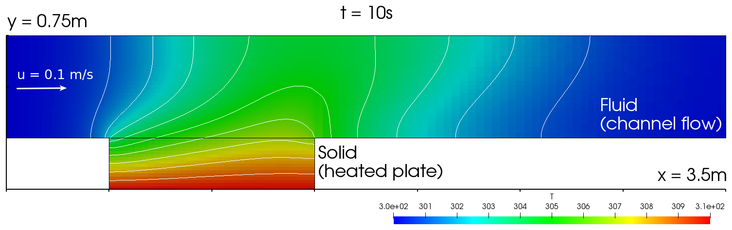
Key pointsPerkara utama
- The unknown is a field T(x, y); FEM solves for nodal values and interpolates between them.Unknown ialah field T(x, y); FEM menyelesaikan nilai pada node dan interpolate di antaranya.
- FEM adds no physics; it turns a PDE into [K]{T̂} = {r}.FEM tidak menambah fizik; ia menukar PDE kepada [K]{T̂} = {r}.
- Scalar field: one unknown per node. Plane stress will have two.Scalar field: satu unknown setiap node. Plane stress akan ada dua.
Quick check · not gradedSemak cepat · tidak bergred
What does the finite element method add to the physics of heat conduction?Apa yang finite element method tambah kepada fizik heat conduction?
Nothing. The physics is the energy balance and Fourier’s law; FEM is a numerical method that turns the resulting PDE into algebraic equations.Tiada apa-apa. Fiziknya ialah energy balance dan Fourier’s law; FEM ialah kaedah berangka yang menukar PDE itu kepada algebraic equation.
2. From the energy balance to the PDEDaripada energy balance kepada PDE
≈ 10 min
Take a small rectangle dx by dy inside the plate, of unit thickness. The dependent variables are the heat fluxes qx and qy (W m−2): energy per unit time per unit area crossing a face. Heat enters through the near faces and leaves through the far faces.Ambil satu segi empat kecil dx × dy di dalam plat, dengan ketebalan unit. Dependent variable ialah heat flux qx dan qy (W m−2): tenaga per unit masa per unit luas yang melintasi satu muka. Haba masuk melalui muka dekat dan keluar melalui muka jauh.
The flux on the far face is the near-face flux plus its change across the element, a first-order Taylor expansion. The net inflow in the x-direction is thereforeFlux pada muka jauh ialah flux muka dekat ditambah perubahannya merentasi element, iaitu first-order Taylor expansion. Jadi net inflow dalam arah x ialah
(2.2)
and by the same argument in the y-directiondan dengan hujah yang sama dalam arah y
(2.3)
Inside, heat is generated at a rate qh per unit volume (W m−3), for example the hydration of cement, and the element stores energy as its temperature rises:Di dalam, haba dijana pada kadar qh per unit isi padu (W m−3), contohnya hydration simen, dan element menyimpan tenaga apabila temperature-nya naik:
(2.5)
(2.1)
Conservation of energyConservation of energy
Rate of change of stored energy = net conduction in + heat generated. Every term carries the factor dx dy, the volume of the element per unit thickness, so it cancels:Kadar perubahan tenaga tersimpan = net conduction masuk + haba dijana. Setiap term membawa faktor dx dy, iaitu isi padu element per unit ketebalan, jadi ia terbatal:
(2.6)
Per unit thicknessPer unit ketebalanEvery quantity is multiplied by the same thickness t, which cancels, so we take t = 1. Nothing changes for a plate of any thickness as long as the faces are insulated.Setiap kuantiti didarab dengan ketebalan t yang sama, yang terbatal, jadi kita ambil t = 1. Tiada yang berubah untuk plat setebal mana pun selagi mukanya insulated.
Fourier’s law closes the systemFourier’s law melengkapkan sistem
The balance has three unknowns (T, qx, qy) and one equation. Fourier’s law supplies the other two: heat flows down the temperature gradient, in proportion to the conductivity k (W m−1 K−1). The minus sign is the physics: flux points from hot to cold.Balance ini ada tiga unknown (T, qx, qy) dan satu persamaan. Fourier’s law membekalkan dua lagi: haba mengalir menuruni temperature gradient, berkadar dengan conductivity k (W m−1 K−1). Tanda negatif itulah fiziknya: flux menghala dari panas ke sejuk.
(2.7)
Substituting (2.7) into the balance gives one equation in T alone:Menggantikan (2.7) ke dalam balance memberi satu persamaan dalam T sahaja:
(2.10)
Steady state: the PDE we discretiseSteady state: PDE yang kita discretise
Drop the time derivative. This is the equation you must be able to write from memory: the divergence of the flux equals the source.Gugurkan time derivative. Inilah persamaan yang anda mesti boleh tulis tanpa melihat nota: divergence bagi flux sama dengan source.
(2.11)
Two special cases you have met before: with constant isotropic k it is Poisson’s equation, and with no source it is Laplace’s equation — the same equation as potential flow in fluid mechanics and seepage in soil mechanics.Dua kes khas yang anda pernah temui: dengan k yang constant dan isotropic ia menjadi Poisson’s equation, dan tanpa source ia menjadi Laplace’s equation — persamaan yang sama dengan potential flow dalam mekanik bendalir dan seepage dalam mekanik tanah.
Unit checkSemakan unitEach term of (2.11) is W m−3: (W m−1 K−1)(K m−2). The source qh sits on the right with a minus sign because we moved it across; a positive source makes the field concave, a hill.Setiap term dalam (2.11) ialah W m−3: (W m−1 K−1)(K m−2). Source qh berada di kanan dengan tanda negatif kerana kita pindahkannya; source positif menjadikan field itu concave, seperti bukit.
The matrix form we will reuseBentuk matrix yang akan kita guna semula
Write the operator as a row of derivatives, a material matrix and a column of derivatives. This is the slide that pays off in plane stress, where the same pattern appears with a 3 × 3 [E] and a 2 × 3 operator.Tulis operator sebagai satu baris derivative, satu material matrix dan satu lajur derivative. Inilah bentuk yang membuahkan hasil dalam plane stress, apabila pola yang sama muncul dengan [E] 3 × 3 dan operator 2 × 3.
(2.12)
(2.13)
(2.14)
Order mattersSusunan penting{∂} is a row of operators, not numbers: it acts on whatever stands to its right. You cannot commute it past a function.{∂} ialah satu baris operator, bukan nombor: ia bertindak ke atas apa sahaja di sebelah kanannya. Anda tidak boleh menukar susunannya melepasi sesuatu fungsi.
Worked step · the y-direction balance (Activity 2)Langkah bekerja · balance arah y (Aktiviti 2)
In through y = 0: qy dx. Out through y = dy: (qy + ∂qy/∂y dy) dx. Net inflow Qy = −∂qy/∂y dx dy, equation (2.3). Add Qx, Qy and Qh, set the sum equal to the stored-energy rate QE, cancel dx dy, and (2.6) follows.Masuk melalui y = 0: qy dx. Keluar melalui y = dy: (qy + ∂qy/∂y dy) dx. Net inflow Qy = −∂qy/∂y dx dy, persamaan (2.3). Tambah Qx, Qy dan Qh, samakan hasil tambahnya dengan kadar tenaga tersimpan QE, batalkan dx dy, dan (2.6) terhasil.
Key pointsPerkara utama
- Energy balance on dx × dy, then Fourier’s law, gives (2.11): divergence of flux = source.Energy balance pada dx × dy, kemudian Fourier’s law, memberi (2.11): divergence flux = source.
- Every term of (2.11) is W m−3.Setiap term dalam (2.11) ialah W m−3.
- Matrix form {∂}[E]{∂}ᵀT = −qh; [E] = diag(kx, ky).Bentuk matrix {∂}[E]{∂}ᵀT = −qh; [E] = diag(kx, ky).
Quick check · not gradedSemak cepat · tidak bergred
What are the units of the heat-generation term qh in (2.11)?Apakah unit bagi term heat generation qh dalam (2.11)?
qh is heat generated per unit volume, W m−3, the same as k ∂²T/∂x². A flux (W m−2) is per unit area; conductivity is W m−1 K−1.qh ialah haba dijana per unit isi padu, W m−3, sama dengan k ∂²T/∂x². Flux (W m−2) ialah per unit luas; conductivity ialah W m−1 K−1.
3. Boundary conditions: essential and naturalBoundary condition: essential dan natural
≈ 7 min
A PDE alone is not a problem. On every part of the boundary we must specify either the temperature or the flux. There are only two kinds of condition, and the whole of the finite element treatment depends on telling them apart.PDE sahaja bukan satu masalah. Pada setiap bahagian sempadan kita mesti tetapkan sama ada temperature atau flux. Hanya ada dua jenis condition, dan keseluruhan rawatan finite element bergantung pada kebolehan membezakannya.
(2.16)
(2.15)
Dirichlet, or essentialDirichlet, atau essentialThe temperature T̄ is known on the edge. FEM must impose it on the unknowns: the corresponding rows and columns of the assembled system are modified.Temperature T̄ diketahui pada tepi itu. FEM mesti mengenakannya pada unknown: baris dan lajur yang sepadan dalam assembled system diubah suai.
Neumann, or naturalNeumann, atau naturalThe boundary flux qb is known, positive inward, and enters through the outward unit normal n = (nx, ny). FEM does not impose it: it appears by itself as a load, from the integration by parts in Part 2.Boundary flux qb diketahui, positif ke dalam, dan masuk melalui outward unit normal n = (nx, ny). FEM tidak mengenakannya: ia muncul dengan sendirinya sebagai load, daripada integration by parts dalam Part 2.
Rectangular domainsRectangular domain
On a rectangle the normal is one of (±1, 0) or (0, ±1), so (2.15) loses one term on every edge:Pada segi empat tepat, normal ialah salah satu daripada (±1, 0) atau (0, ±1), jadi (2.15) kehilangan satu term pada setiap tepi:
What FEM does with each kindApa yang FEM buat dengan setiap jenis
| ConditionCondition | What is knownApa yang diketahui | Where it enters the FEMDi mana ia masuk dalam FEM | Action in Part 2Tindakan dalam Part 2 |
|---|---|---|---|
| Dirichlet · essential | T̄ on the edgepada tepi | imposed on the assembled system by modifying rows and columns of [K]dikenakan pada assembled system dengan mengubah baris dan lajur [K] | row–column eliminationrow–column elimination |
| Neumann · natural | qb on the edgepada tepi | appears in the boundary vector {b} produced by integration by partsmuncul dalam boundary vector {b} hasil integration by parts | {b} = ∫{N}ᵀqn ds |
| Insulated · natural, qb = 0Insulated · natural, qb = 0 | no fluxtiada flux | contributes nothing: the boundary integral is zerotiada sumbangan: boundary integral sifar | do nothingtiada tindakan |
The most common errorKesilapan paling lazimTrying to “impose” an insulated edge. It needs no action at all. The names come from the integration by parts: the natural condition is the term that falls out of it; the essential one must be enforced on the unknowns.Cuba “mengenakan” tepi insulated. Ia tidak memerlukan apa-apa tindakan. Nama-namanya datang daripada integration by parts: natural condition ialah term yang terhasil daripadanya; essential condition mesti dikuatkuasakan pada unknown.
Worked example · label the plate (Activity 3, text Exercise 2.5)Contoh bekerja · label plat (Aktiviti 3, teks Latihan 2.5)
| EdgeTepi | TypeJenis | EquationPersamaan | FEM actionTindakan FEM |
|---|---|---|---|
| topatas | Dirichlet | T = 300 K | impose on the systemkenakan pada sistem |
| leftkiri | Dirichlet | T = 400 K | impose on the systemkenakan pada sistem |
| rightkanan | Neumann | n = (1, 0): k ∂T/∂x = qb = +1 × 10⁶ W m−2 | load in {b}load dalam {b} |
| bottombawah | Neumann, qb = 0 | ∂T/∂y = 0 | nothingtiada |
Well-posed: every edge has a condition and T is fixed on two edges, so the temperature level is pinned. The inward flux on the right edge is positive qb; the flux-vector component qx there points along −n and is negative, qx = −106 W m−2.Well-posed: setiap tepi ada condition dan T ditetapkan pada dua tepi, jadi paras temperature terikat. Flux ke dalam pada tepi kanan ialah qb positif; komponen flux-vector qx di situ menghala sepanjang −n dan negatif, qx = −106 W m−2.
Key pointsPerkara utama
- Dirichlet = essential = imposed. Neumann = natural = appears from the integration by parts. Insulated = do nothing.Dirichlet = essential = dikenakan. Neumann = natural = muncul daripada integration by parts. Insulated = tiada tindakan.
- qb is positive inward; on a rectangle only one derivative survives per edge.qb positif ke dalam; pada segi empat tepat hanya satu derivative kekal pada setiap tepi.
- A problem is well-posed when every edge has a condition and T is pinned somewhere.Masalah itu well-posed apabila setiap tepi ada condition dan T terikat di suatu tempat.
Quick check · not gradedSemak cepat · tidak bergred
An edge of the plate is insulated. In the finite element model, what must you do about it?Satu tepi plat adalah insulated. Dalam model finite element, apa yang anda perlu buat?
An insulated edge is a natural condition with qb = 0, so the boundary term {b} it would produce is zero. No action is needed.Tepi insulated ialah natural condition dengan qb = 0, jadi boundary term {b} yang bakal dihasilkannya ialah sifar. Tiada tindakan diperlukan.
4. The four-node element and its shape functionsFour-node element dan shape function-nya
≈ 12 min
The four-node rectangular element has one degree of freedom at each corner, the temperature T̂i, numbered anticlockwise from the bottom-left corner. We need a rule for T at any point inside the element in terms of these four numbers. The rule is a polynomial with four coefficients.Four-node rectangular element mempunyai satu degree of freedom pada setiap bucu, iaitu temperature T̂i, dinomborkan lawan jam dari bucu kiri bawah. Kita perlukan satu peraturan bagi T pada mana-mana titik di dalam element dalam sebutan empat nombor ini. Peraturannya ialah satu polynomial dengan empat coefficient.
Step 1 · assume a polynomial (2.17)Langkah 1 · andaikan satu polynomial (2.17)
(2.17)
Four unknowns need four coefficients. The xy term, rather than x² or y², keeps the function linear along every edge, which is what makes neighbouring elements agree.Empat unknown memerlukan empat coefficient. Term xy, bukannya x² atau y², mengekalkan fungsi itu linear di sepanjang setiap tepi, dan itulah yang membuat element berjiran bersetuju.
Step 2 · evaluate at the nodes (2.18)Langkah 2 · nilaikan pada node (2.18)
(2.18)
Step 3 · solve for the coefficients (2.19)Langkah 3 · selesaikan coefficient (2.19)
(2.19)
Check: if all four nodal values are equal to T0, then a1 = T0 and a2 = a3 = a4 = 0, so T = T0 everywhere. A uniform field is reproduced exactly.Semak: jika keempat-empat nilai node sama dengan T0, maka a1 = T0 dan a2 = a3 = a4 = 0, jadi T = T0 di mana-mana. Field yang seragam dihasilkan semula dengan tepat.
Step 4 · collect by nodal value (2.20)–(2.22)Langkah 4 · kumpulkan mengikut nilai node (2.20)–(2.22)
(2.20)
(2.21)
(2.22)
Each nodal value is multiplied by its own function of position: its shape function Ni(x, y). The row {N} and the column {T̂}ᵀ are the two objects the rest of the course is built from.Setiap nilai node didarab dengan fungsi kedudukannya sendiri: shape function Ni(x, y). Baris {N} dan lajur {T̂}ᵀ ialah dua objek yang menjadi asas keseluruhan kursus ini.
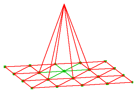
What a shape function looks likeRupa sebuah shape function
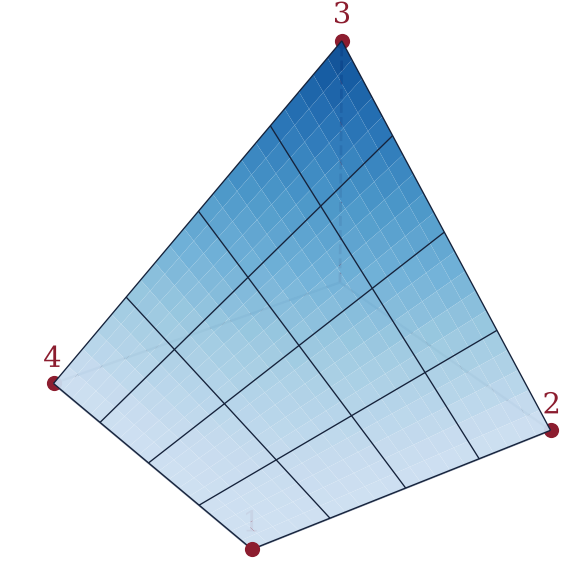
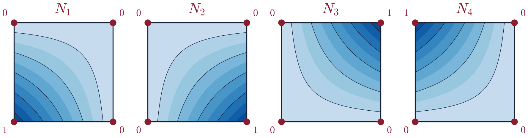
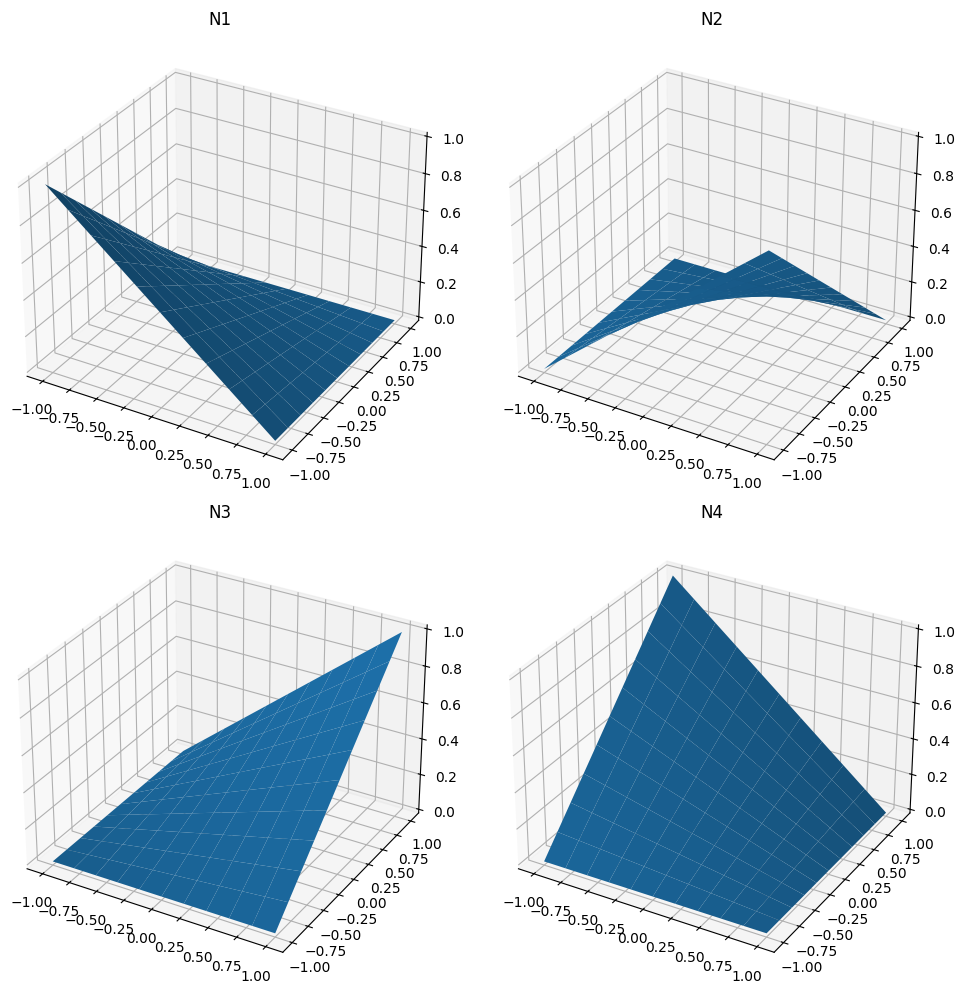
Three properties you can check in 30 secondsTiga sifat yang boleh disemak dalam 30 saat
Kronecker delta. So T at node j equals T̂j: the nodal unknowns really are nodal temperatures. Check N2 at node 3: N2(a, b) = a(b − b)/(ab) = 0.Kronecker delta. Jadi T pada node j sama dengan T̂j: nodal unknown memang temperature pada node. Semak N2 pada node 3: N2(a, b) = a(b − b)/(ab) = 0.
Partition of unity. A uniform temperature is reproduced exactly, the test we did on the coefficients.Partition of unity. Temperature yang seragam dihasilkan semula dengan tepat, ujian yang kita buat pada coefficient tadi.
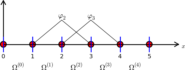
Linear along each edge. On y = 0 only nodes 1 and 2 matter, and T varies linearly between them. The neighbouring element shares those two nodes and the same straight line, so T is continuous across element boundaries (C0).Linear di sepanjang setiap tepi. Pada y = 0 hanya node 1 dan 2 yang penting, dan T berubah secara linear antara keduanya. Element berjiran berkongsi dua node itu dan garis lurus yang sama, jadi T adalah continuous merentasi sempadan element (C0).
From one element to the meshDaripada satu element kepada mesh
Worked example · evaluate and interpolate (Activity 4)Contoh bekerja · nilaikan dan interpolate (Aktiviti 4)
a = 2 m, b = 1 m, point (x, y) = (1.5, 0.3) m, nodal temperatures T̂ = {100, 140, 160, 120} K.a = 2 m, b = 1 m, titik (x, y) = (1.5, 0.3) m, nodal temperature T̂ = {100, 140, 160, 120} K.
Node 2 carries half the weight because the point is nearest to it. The sum of the four weights is 1, as it must be.Node 2 membawa separuh daripada weight kerana titik itu paling hampir dengannya. Hasil tambah empat weight ialah 1, sebagaimana sepatutnya.
Key pointsPerkara utama
- T = {N}{T̂}ᵀ with the bilinear Ni of (2.21).T = {N}{T̂}ᵀ dengan Ni bilinear daripada (2.21).
- Kronecker delta, partition of unity, linear edges: three checks that catch most errors.Kronecker delta, partition of unity, tepi linear: tiga semakan yang menangkap kebanyakan kesilapan.
- At (1.5, 0.3): N = 0.175, 0.525, 0.225, 0.075 and T = 136.0 K.Pada (1.5, 0.3): N = 0.175, 0.525, 0.225, 0.075 dan T = 136.0 K.
Quick check · not gradedSemak cepat · tidak bergred
At the centre of the element (a/2, b/2), what is the value of each shape function?Pada pusat element (a/2, b/2), apakah nilai setiap shape function?
Ni(a/2, b/2) = (a/2)(b/2)/(ab) = 1/4 for every i, and the four values sum to 1.Ni(a/2, b/2) = (a/2)(b/2)/(ab) = 1/4 bagi setiap i, dan empat nilai itu berjumlah 1.
5. Gradient and flux inside an elementGradient dan flux di dalam element
≈ 7 min
Differentiate the approximation T = {N}{T̂}ᵀ and the derivatives land on the shape functions, because the nodal values are constants. The gradient at any point is a 2 × 4 matrix of shape-function derivatives times the nodal vector:Bezakan approximation T = {N}{T̂}ᵀ dan derivative itu jatuh pada shape function, kerana nilai node ialah pemalar. Gradient pada mana-mana titik ialah matrix 2 × 4 bagi derivative shape function didarab dengan nodal vector:
(2.33)
Read the matrix: ∂Ni/∂x depends on y only and ∂Ni/∂y on x only. Across an element edge the gradient, and therefore the flux, generally jumps — the approximation is continuous but its derivative is not.Baca matrix itu: ∂Ni/∂x bergantung pada y sahaja dan ∂Ni/∂y pada x sahaja. Merentasi tepi element, gradient dan seterusnya flux biasanya melompat — approximation itu continuous tetapi derivative-nya tidak.
From gradient to fluxDaripada gradient kepada flux
Fourier’s law in matrix form: flux = −[E] × gradient. The same 2 × 4 matrix {∂}ᵀ{N} will be used twice: for the flux now, and for the conductance matrix in Part 2:Fourier’s law dalam bentuk matrix: flux = −[E] × gradient. Matrix 2 × 4 yang sama, {∂}ᵀ{N}, akan digunakan dua kali: untuk flux sekarang, dan untuk conductance matrix dalam Part 2:
Worked example · gradient and flux at (1.5, 0.3) (Activity 5)Contoh bekerja · gradient dan flux pada (1.5, 0.3) (Aktiviti 5)
Same element and data as Activity 4, with kx = ky = 2 W m−1 K−1.Element dan data yang sama dengan Aktiviti 4, dengan kx = ky = 2 W m−1 K−1.
Both components of the flux are negative: heat flows towards decreasing x and y, away from the hottest node 3 at (a, b).Kedua-dua komponen flux negatif: haba mengalir ke arah x dan y yang menyusut, menjauhi node 3 yang paling panas di (a, b).
The eight-node element in one paragraphEight-node element dalam satu perenggan
Add a node at the middle of each edge and the polynomial gains four terms, (2.31). The shape functions are quadratic along each edge, so they follow a curved temperature profile with fewer elements. The procedure is identical: evaluate at the eight nodes, invert, collect by nodal value. A corner function now dips below zero between its two mid-side neighbours, and the eight functions still sum to one.Tambah satu node di tengah setiap tepi dan polynomial itu mendapat empat term lagi, (2.31). Shape function-nya quadratic di sepanjang setiap tepi, jadi ia mengikut profil temperature yang melengkung dengan element yang lebih sedikit. Prosedurnya serupa: nilaikan pada lapan node, inverse, kumpulkan mengikut nilai node. Fungsi bucu kini jatuh di bawah sifar antara dua jiran tengah sisinya, dan lapan fungsi itu tetap berjumlah satu.
(2.31)
Key pointsPerkara utama
- Gradient = {∂}ᵀ{N}{T̂}ᵀ, a 2 × 4 matrix times the nodal vector; flux = −[E] × gradient.Gradient = {∂}ᵀ{N}{T̂}ᵀ, matrix 2 × 4 didarab nodal vector; flux = −[E] × gradient.
- At (1.5, 0.3) with k = 2: ∂T/∂x = ∂T/∂y = 20 K m−1, qx = qy = −40 W m−2.Pada (1.5, 0.3) dengan k = 2: ∂T/∂x = ∂T/∂y = 20 K m−1, qx = qy = −40 W m−2.
- The eight-node element is the same procedure with quadratic edges.Eight-node element ialah prosedur yang sama dengan tepi quadratic.
Quick check · not gradedSemak cepat · tidak bergred
At a point the temperature increases in the +x direction. The flux component qx there isPada satu titik, temperature meningkat dalam arah +x. Komponen flux qx di situ ialah
qx = −k ∂T/∂x. A positive gradient gives a negative flux: heat flows from hot to cold, towards −x.qx = −k ∂T/∂x. Gradient positif memberi flux negatif: haba mengalir dari panas ke sejuk, ke arah −x.
6. The pipeline: seven steps from PDE to answerPipeline: tujuh langkah daripada PDE kepada jawapan
≈ 5 min
The method is a pipeline of seven steps. This part covered the first two; Part 2 does the other five on the text’s worked example and runs the MATLAB script.Kaedah ini ialah satu pipeline tujuh langkah. Bahagian ini merangkumi dua langkah pertama; Part 2 membuat lima lagi pada contoh bekerja dalam teks dan menjalankan skrip MATLAB.
- Governing PDE and boundary conditionsPDE pentadbir dan boundary condition · this partbahagian ini
- Element and shape functionsElement dan shape function · this partbahagian ini
- Galerkin weighted residualGalerkin weighted residual
- Integration by partsIntegration by parts
- Element matrices [k], {q}, {b}Matrix element [k], {q}, {b}
- Assembly, then impose T̄Assembly, kemudian kenakan T̄
- Solve and post-processSelesaikan dan post-process
Part 2’s worked example (text §2.3)Contoh bekerja Part 2 (teks §2.3)
Square plate 1 m × 1 m, qh = 600 W m−3, kx = ky = 300 W m−1 K−1; top and left edges at 0 °C, right and bottom edges insulated. Four 4-node elements by hand, then 64 elements in MATLAB, then software.Plat segi empat sama 1 m × 1 m, qh = 600 W m−3, kx = ky = 300 W m−1 K−1; tepi atas dan kiri pada 0 °C, tepi kanan dan bawah insulated. Empat 4-node element secara tangan, kemudian 64 element dalam MATLAB, kemudian perisian.
Before Part 2Sebelum Part 2Classify its four edges as in §3 and predict where the hottest point is. Write the prediction down; Part 2 checks it.Kelaskan empat tepinya seperti dalam §3 dan ramalkan di mana titik paling panas. Tulis ramalan itu; Part 2 menyemaknya.
The MATLAB skeleton follows the pipelineRangka MATLAB mengikut pipeline
% Local conductance matrix (text §2.3.1)
a = L/Nx; b = H/Ny;
s1 = b*kx/(3*a) + a*ky/(3*b);
s2 = -b*kx/(3*a) + a*ky/(6*b);
s3 = -b*kx/(6*a) - a*ky/(6*b);
s4 = b*kx/(6*a) - a*ky/(3*b);
k = [s1 s2 s3 s4; s2 s1 s4 s3; s3 s4 s1 s2; s4 s3 s2 s1];
fQ = a*b*Q/4*[1; 1; 1; 1];        % heat generation
% Assembly by connectivity, element 1 = nodes [1 2 5 4]
e1 = [1 2 5 4];  K(e1,e1) = K(e1,e1) + k;  F(e1) = F(e1) + fQ;
% Essential conditions: rows and columns of known nodes removed
free = setdiff(1:n, fixed);  T = zeros(n,1);  T(fixed) = Tbar;
T(free) = K(free,free) \ (F(free) - K(free,fixed)*T(fixed));
- Lines 2–8: step 5, the element matrix and load from closed-form integrals (s1…s4 are derived in Part 2).Baris 2–8: langkah 5, matrix element dan load daripada closed-form integral (s1…s4 diterbitkan dalam Part 2).
- Line 10: step 6, assembly — the connectivity list [1 2 5 4] is the element’s global node numbers.Baris 10: langkah 6, assembly — senarai connectivity [1 2 5 4] ialah nombor node global bagi element itu.
- Lines 12–13: step 6, essential conditions by removing the rows and columns of the known nodes; step 7, solve with the backslash operator.Baris 12–13: langkah 6, essential condition dengan membuang baris dan lajur node yang diketahui; langkah 7, selesaikan dengan operator backslash.
To preparePersediaan
- Read text §2.2.2 and §2.3 (the worked example), about 12 pages.Baca teks §2.2.2 dan §2.3 (contoh bekerja), kira-kira 12 muka surat.
- Redo Activities 4 and 5 for the point (0.5, 0.8) m — or use the exercises tab, which gives you new numbers each time.Ulang Aktiviti 4 dan 5 untuk titik (0.5, 0.8) m — atau guna tab Latihan, yang memberi nombor baharu setiap kali.
- Classify the edges of the §2.3 plate and predict the hottest point.Kelaskan tepi plat §2.3 dan ramalkan titik paling panas.
- Bring MATLAB to the next session.Bawa MATLAB ke sesi seterusnya.
Key pointsPerkara utama
- Seven steps: PDE + BCs, element, Galerkin, integration by parts, element matrices, assembly + impose, solve.Tujuh langkah: PDE + BC, element, Galerkin, integration by parts, matrix element, assembly + kenakan, selesaikan.
- Part 2: steps 3–7 on the 1 m plate, by hand with four elements and in MATLAB with 64.Part 2: langkah 3–7 pada plat 1 m, secara tangan dengan empat element dan dalam MATLAB dengan 64.
Quick check · not gradedSemak cepat · tidak bergred
For the §2.3 plate (cold top and left edges, insulated right and bottom edges, uniform heat generation), where is the hottest point?Bagi plat §2.3 (tepi atas dan kiri sejuk, tepi kanan dan bawah insulated, heat generation seragam), di manakah titik paling panas?
Heat can only leave through the two cold edges. The point farthest from both, where the two insulated edges meet, is the bottom-right corner.Haba hanya boleh keluar melalui dua tepi sejuk. Titik yang paling jauh daripada kedua-duanya, tempat dua tepi insulated bertemu, ialah bucu kanan bawah.

SlidesSlides
What to doApa perlu dibuat Step through with ◀ ▶ (⏮ ⏭ for the first and last), the ← → keys, the mouse wheel or a swipe on the slide, or drag the bar under the slide to any page; the list below jumps to any slide. Download the PDF for printing and offline reading.Gerak dengan ◀ ▶ (⏮ ⏭ untuk slide pertama dan terakhir), kekunci ← →, roda tetikus atau leret pada slide, atau seret bar di bawah slide ke mana-mana halaman; senarai di bawah melompat ke mana-mana slide. Muat turun PDF untuk cetakan dan bacaan luar talian.
Counts toward progress:Dikira dalam kemajuan: each slide you open, once.setiap slide yang anda buka, sekali.
Loading slides…Memuatkan slides…

ExamplesContoh
What to doApa perlu dibuat Model answers in exam form, with suggested marks. Try each question on paper first, then compare step by step; tick it at the end when you have worked through it.Jawapan model dalam bentuk peperiksaan, dengan markah cadangan. Cuba setiap soalan di atas kertas dahulu, kemudian bandingkan langkah demi langkah; tandanya di hujung apabila anda sudah mengikutinya.
Counts toward progress:Dikira dalam kemajuan: examples ticked as worked through.contoh yang ditanda sudah diikuti.
How this topic is examinedBagaimana topik ini diuji
Model answers in the form the examiner expects: physical picture, plan, numbered steps with every substitution written out, checks, a boxed answer and an interpretation. The marks shown are a suggested scheme for a 20-mark question; the examiner’s own scheme may differ.Jawapan model dalam bentuk yang pemeriksa jangkakan: gambaran fizikal, pelan, langkah bernombor dengan setiap penggantian ditulis, semakan, jawapan berkotak dan tafsiran. Markah yang ditunjukkan ialah skema cadangan untuk soalan 20 markah; skema pemeriksa sendiri mungkin berbeza.
| Question typeJenis soalan | Given and wantedDiberi dan dikehendaki | Plan and the usual trapPelan dan perangkap biasa |
|---|---|---|
| Shape functionsShape function | Node coordinates and the interpolation polynomial; wanted: Ni.Koordinat node dan polynomial interpolation; dikehendaki: Ni. | Nodal conditions, solve for ai, collect the Ti. Trap: no check of Ni = 1 at node i and 0 at the others.Nodal condition, selesaikan ai, kumpulkan Ti. Perangkap: tiada semakan Ni = 1 pada node i dan 0 pada node lain. |
| Temperature at a pointTemperature pada satu titik | Nodal temperatures; wanted: T(x, y), sometimes the flux.Nodal temperature; dikehendaki: T(x, y), kadang-kadang flux. | Find the element, use its local coordinates in Ni. Trap: global x, y in Ni.Cari element, guna koordinat local dalam Ni. Perangkap: x, y global dalam Ni. |
| ExplainTerangkan | Imposing T = T̄; insulated edges; why a row adds up to zero.Mengenakan T = T̄; tepi insulated; mengapa satu baris berjumlah sifar. | Claim, reason, consequence — three sentences, in that order.Dakwaan, sebab, akibat — tiga ayat, mengikut urutan itu. |
Notation follows the companion: Q is the heat generated per unit volume (the text’s qh), qn the inward boundary flux (the text’s qb), t the thickness.Notasi mengikut buku pendamping: Q ialah haba dijana per unit isi padu (qh dalam teks), qn boundary flux ke dalam (qb dalam teks), t ketebalan.
Example 1 · Shape functions and conductance matrix of a triangleContoh 1 · Shape function dan conductance matrix bagi segi tiga
QuestionSoalanA three-node heat element has its nodes at (0, 0), (L, 0) and (L/2, L). With the interpolation T(x, y) = a1 + a2x + a3y, (a) derive the shape functions by writing T = N1T1 + N2T2 + N3T3, (b) check them, and (c) find the conductance matrix for kx = ky = k and thickness t.
Physical picture.Gambaran fizikal. A plane over a triangle is fixed by its three corner values, so the three nodal temperatures determine a1, a2 and a3. Each shape function is the field obtained with its own node at 1 and the other two at 0: a plane that is 1 at that node and 0 along the opposite side. Side 1–2 lies on y = 0, so N3 must depend on y only.Satah di atas segi tiga ditentukan oleh tiga nilai bucunya, jadi tiga nodal temperature menentukan a1, a2 dan a3. Setiap shape function ialah field yang diperoleh dengan node sendiri bernilai 1 dan dua node lain 0: satah yang bernilai 1 pada node itu dan 0 di sepanjang sisi bertentangan. Sisi 1–2 terletak pada y = 0, jadi N3 mesti bergantung pada y sahaja.
Plan. Three nodal conditions → a1, a2, a3 → collect T1, T2, T3 → checks → derivatives → [k].
Step 1 Nodal conditionsNodal condition[3]
Step 2 (a) The coefficients(a) Coefficient[3]
From the first two, a1 = T1 and a2 = (T2 − T1)/L. The third then givesDaripada dua yang pertama, a1 = T1 dan a2 = (T2 − T1)/L. Yang ketiga kemudian memberi
Step 3 Collecting the nodal temperaturesMengumpul nodal temperature[2]
Answer. (a)
Step 4 (b) Checks(b) Semakan[3]
Nodes 1 and 2 check in the same way. At the centroid (L/2, L/3) each function is 1/3.Node 1 dan 2 disemak dengan cara yang sama. Pada centroid (L/2, L/3) setiap fungsi bernilai 1/3.
Answer. (b) Ni = 1 at node i and 0 at the others; ΣNi = 1 everywhere.
Step 5 (c) Derivatives and [k](c) Derivative dan [k][9]
The derivatives are constant, so the integral kij = t∫(kx Ni,xNj,x + ky Ni,yNj,y) dA is the area times the integrand (the conductance matrix of Part 2):Derivative itu pemalar, jadi integral kij = t∫(kx Ni,xNj,x + ky Ni,yNj,y) dA ialah luas didarab integrand (conductance matrix dalam Part 2):
Answer. (c)
each row adds up to zero.
Check. Row 1: 5 − 3 − 2 = 0; row 3: −2 − 2 + 4 = 0. [k] is symmetric.
InterpretationTafsiran[k] does not contain L. Each entry is the thickness times the area, which grows as L², times a product of two gradients, each of which falls as 1/L; the two effects cancel, so a triangle of the same shape conducts the same heat per kelvin whatever its size. Every row adds up to zero because a uniform temperature, T1 = T2 = T3, produces no heat flow. The temperature inside the element is a plane, so its gradient, and with it the heat flux, is constant in each element and jumps from one element to the next; the temperature itself stays continuous, since along a shared side it varies linearly between the same two nodal values.[k] tidak mengandungi L. Setiap entri ialah ketebalan didarab luas, yang membesar sebagai L², didarab hasil darab dua gradient yang masing-masing menyusut sebagai 1/L; dua kesan itu saling membatalkan, jadi segi tiga dengan bentuk yang sama mengalirkan haba yang sama per kelvin tanpa mengira saiznya. Setiap baris berjumlah sifar kerana temperature seragam, T1 = T2 = T3, tidak menghasilkan aliran haba. Temperature di dalam element ialah satah, jadi gradient-nya, dan seterusnya heat flux, adalah pemalar dalam setiap element dan melompat dari satu element ke element seterusnya; temperature itu sendiri kekal continuous, kerana di sepanjang sisi yang dikongsi ia berubah secara linear antara dua nilai node yang sama.
Marking scheme (suggested)Skema pemarkahan (cadangan) · 20
| What earns the marksApa yang diberi markah | MarksMarkah |
|---|---|
| Three nodal conditions written correctlyTiga nodal condition ditulis dengan betul | 3 |
| a1, a2, a3a1, a2, a3 | 3 |
| Collecting by nodal value → N1, N2, N3Mengumpul mengikut nilai node → N1, N2, N3 | 2 |
| Kronecker and partition-of-unity checksSemakan Kronecker dan partition of unity | 3 |
| Derivative vectors and the areaVektor derivative dan luas | 3 |
| Three entries by integration, matrix by symmetry, row-sum checkTiga entri melalui integration, matrix melalui simetri, semakan jumlah baris | 6 |
| TotalJumlah | 20 |
Example 2 · Temperature and flux at a point of a four-node elementContoh 2 · Temperature dan flux pada satu titik four-node element
QuestionSoalanA four-node element 0.4 m by 0.3 m has nodal temperatures 20, 40, 60 and 30 °C at nodes 1 to 4 (anticlockwise from the origin), and k = 15 W m−1 K−1. Find T, qx and qy (a) at the centre and (b) at the local point (0.1, 0.2) m.
Physical picture.Gambaran fizikal. The nodal values rise from node 1 to node 3, so the temperature increases in both +x and +y; Fourier’s law then makes both flux components negative, pointing back towards node 1. The gradient of a bilinear field is not constant: ∂T/∂x changes with y and ∂T/∂y with x, so the two points will give different fluxes.Nilai node meningkat dari node 1 ke node 3, jadi temperature bertambah dalam arah +x dan +y; Fourier’s law kemudian menjadikan kedua-dua komponen flux negatif, menghala kembali ke node 1. Gradient bagi field bilinear tidak malar: ∂T/∂x berubah dengan y dan ∂T/∂y dengan x, jadi dua titik itu akan memberi flux yang berbeza.
Plan. Ni at the point → T = ΣNiTi → ∂Ni/∂x, ∂Ni/∂y from (2.33) → gradient → q = −k∇T. ab = 0.4 × 0.3 = 0.12 m² throughout.
Step 1 (a) Shape functions and T at the centre(a) Shape function dan T pada pusat[4]
Step 2 (a) Derivatives at the centre (y = 0.15, x = 0.2)(a) Derivative pada pusat (y = 0.15, x = 0.2)[3]
Step 3 (a) Gradient and flux at the centre(a) Gradient dan flux pada pusat[3]
Answer. (a) T = 37.5 °C; qx = −938 W m−2, qy = −750 W m−2.
Check. ΣNi = 1. Both fluxes negative, as the physical picture predicted.
Step 4 (b) Shape functions and T at (0.1, 0.2)(b) Shape function dan T pada (0.1, 0.2)[5]
With a − x = 0.3 and b − y = 0.1:Dengan a − x = 0.3 dan b − y = 0.1:
Step 5 (b) Gradient and flux at (0.1, 0.2)(b) Gradient dan flux pada (0.1, 0.2)[5]
Answer. (b) T = 33.3 °C; qx = −1000 W m−2, qy = −625 W m−2.
InterpretationTafsiranThe gradient changes between the two points because T1 − T2 + T3 − T4 = 20 − 40 + 60 − 30 = 10 ≠ 0: that combination is the coefficient a4 of the xy term, and it is the only reason the field is not a plane. With four values that sum to zero in that pattern the flux would be the same everywhere in the element. The numbers also show the sign convention at work: a flux is negative when the temperature increases in that direction.Gradient berubah antara dua titik itu kerana T1 − T2 + T3 − T4 = 20 − 40 + 60 − 30 = 10 ≠ 0: gabungan itu ialah coefficient a4 bagi term xy, dan itulah satu-satunya sebab field itu bukan satah. Dengan empat nilai yang berjumlah sifar dalam pola itu, flux akan sama di seluruh element. Nombor-nombor itu juga menunjukkan tanda yang digunakan: flux negatif apabila temperature meningkat dalam arah itu.
Marking scheme (suggested)Skema pemarkahan (cadangan) · 20
| What earns the marksApa yang diberi markah | MarksMarkah |
|---|---|
| Ni = 1/4 at the centre and TNi = 1/4 pada pusat dan T | 4 |
| Derivative rows at the centreBaris derivative pada pusat | 3 |
| Gradient, then q = −k∇T with signsGradient, kemudian q = −k∇T dengan tanda | 3 |
| Ni at (0.1, 0.2), sum check, TNi pada (0.1, 0.2), semakan jumlah, T | 5 |
| Gradient and flux at the pointGradient dan flux pada titik itu | 5 |
| TotalJumlah | 20 |
Example 3 · Explain-type questions: model answersContoh 3 · Soalan jenis terangkan: jawapan model
QuestionsSoalanAnswer each in two or three sentences. State the claim, give the reason, and say what follows from it.Jawab setiap satu dalam dua atau tiga ayat. Nyatakan dakwaan, beri sebab, dan nyatakan apa yang terhasil daripadanya.
Step 1 Why is nothing done at an insulated edge?Mengapa tiada apa-apa dibuat pada tepi insulated?[3]
An insulated edge is a natural condition with qn = 0, so its boundary term t∫{N}qn ds is zero. The Galerkin formulation satisfies it approximately without any action. A non-zero flux would instead enter {r} at the nodes of that edge.Tepi insulated ialah natural condition dengan qn = 0, jadi boundary term-nya t∫{N}qn ds ialah sifar. Formulasi Galerkin memenuhinya secara anggaran tanpa sebarang tindakan. Flux bukan sifar pula akan masuk ke {r} pada node tepi itu.
Step 2 What is the difference between an essential and a natural boundary condition, and how is each imposed?Apakah perbezaan antara essential dan natural boundary condition, dan bagaimana setiap satu dikenakan?[3]
An essential condition prescribes the primary variable, the temperature T = T̄; a natural condition prescribes the secondary variable, the flux qn. The essential condition is imposed on the assembled equations by striking the rows and columns of the known nodes, and the struck rows later give the heat flows there. The natural condition is never imposed: it appears by itself as a load through the boundary term of the integration by parts.Essential condition menetapkan primary variable, iaitu temperature T = T̄; natural condition menetapkan secondary variable, iaitu flux qn. Essential condition dikenakan pada assembled equation dengan membuang baris dan lajur node yang diketahui, dan baris yang dibuang itu kemudian memberi aliran haba di situ. Natural condition tidak pernah dikenakan: ia muncul dengan sendirinya sebagai load melalui boundary term daripada integration by parts.
Step 3 Why does every row of [k] add up to zero, and how is that used?Mengapa setiap baris [k] berjumlah sifar, dan bagaimana ia digunakan?[3]
Since ΣNi = 1, a uniform temperature makes every gradient zero and conducts no heat, so [k]{1, 1, …}ᵀ = {0}. Consequently [k], and an unrestrained [K], are singular, which is why at least one temperature must be prescribed. Every row of a computed matrix can be checked in a few seconds by adding it up.Oleh kerana ΣNi = 1, temperature seragam menjadikan setiap gradient sifar dan tidak mengalirkan haba, jadi [k]{1, 1, …}ᵀ = {0}. Akibatnya [k], dan [K] yang tidak dikekang, adalah singular; sebab itulah sekurang-kurangnya satu temperature mesti ditetapkan. Setiap baris matrix yang dikira boleh disemak dalam beberapa saat dengan menjumlahkannya.
Step 4 How do the three-node and the four-node elements differ?Bagaimana three-node dan four-node element berbeza?[3]
The T3 field is a plane, so its gradient and flux are constant in each element. The Q4 field contains xy, so ∂T/∂x varies with y and ∂T/∂y with x. Both fields vary linearly along every side, so the temperature is continuous between elements while the flux jumps; on the same nodes the Q4 is usually more accurate, but in this course it is limited to rectangles, whereas triangles fit any shape.Field T3 ialah satah, jadi gradient dan flux-nya malar dalam setiap element. Field Q4 mengandungi xy, jadi ∂T/∂x berubah dengan y dan ∂T/∂y dengan x. Kedua-dua field berubah secara linear di sepanjang setiap sisi, jadi temperature continuous antara element manakala flux melompat; pada node yang sama Q4 biasanya lebih tepat, tetapi dalam kursus ini ia terhad kepada segi empat tepat, manakala segi tiga sesuai untuk apa jua bentuk.
InterpretationTafsiranThe examiner looks for the three parts in order. “Insulated means do nothing” alone is a claim without a reason and earns one mark of three; naming the boundary term and its value earns the other two.Pemeriksa mencari tiga bahagian mengikut urutan. “Insulated bermaksud tiada tindakan” sahaja ialah dakwaan tanpa sebab dan mendapat satu daripada tiga markah; menamakan boundary term dan nilainya mendapat dua markah lagi.
Marking scheme (suggested)Skema pemarkahan (cadangan) · 12
| What earns the marksApa yang diberi markah | MarksMarkah |
|---|---|
| Claim stated correctlyDakwaan dinyatakan dengan betul | 1 each |
| Reason: the term, the property or the equation behind itSebab: term, sifat atau persamaan di sebaliknya | 1 each |
| Consequence for the calculationAkibat kepada pengiraan | 1 each |
| TotalJumlah | 12 |

ExercisesLatihan
What to doApa perlu dibuat Start the timer. For each question choose Sure or Not sure first, then answer. The summary at the end compares your confidence with your results.Mulakan timer. Untuk setiap soalan pilih Yakin atau Tak pasti dahulu, kemudian jawab. Ringkasan di hujung membandingkan keyakinan anda dengan keputusan.
Counts toward progress:Dikira dalam kemajuan: questions answered (B: checked, or solution viewed).soalan yang dijawab (B: disemak, atau penyelesaian dilihat).
0:00targetsasaran 30 min · 1.5 min/markmarkah
A Concept questionsSoalan konsep · 6 × 1 markmarkah
Click one option. One try: the right answer is marked ✓ and explained.Klik satu pilihan. Satu cubaan: jawapan betul ditanda ✓ dan diterangkan.
In the steady conduction equation (2.11), which combination has the units of qh?Dalam persamaan steady conduction (2.11), gabungan manakah yang mempunyai unit qh?
Before you answer:Sebelum menjawab:
k ∂²T/∂x² has units (W m−1 K−1)(K m−2) = W m−3, the same as qh. The option k ∂T/∂x is a flux, W m−2.k ∂²T/∂x² berunit (W m−1 K−1)(K m−2) = W m−3, sama dengan qh. Pilihan k ∂T/∂x ialah flux, W m−2.
Which boundary condition must be imposed on the assembled equations rather than appearing by itself?Boundary condition manakah yang mesti dikenakan pada assembled equation dan bukannya muncul dengan sendiri?
Before you answer:Sebelum menjawab:
A known temperature is an essential (Dirichlet) condition: it constrains the unknowns themselves. A known flux, including zero flux, is natural and comes out of the integration by parts.Temperature yang diketahui ialah essential (Dirichlet) condition: ia mengekang unknown itu sendiri. Flux yang diketahui, termasuk flux sifar, adalah natural dan terhasil daripada integration by parts.
On the right edge of a plate, n = (1, 0), an inward flux qb = +500 W m−2 is applied. The flux-vector component qx at that edge isPada tepi kanan plat, n = (1, 0), flux ke dalam qb = +500 W m−2 dikenakan. Komponen flux-vector qx pada tepi itu ialah
Before you answer:Sebelum menjawab:
qb is positive inward. On the right edge, inward means towards −x, so qx = −qb = −500 W m−2. Equivalently (2.15): k ∂T/∂x · nx = qb, so k ∂T/∂x = +500 and qx = −k ∂T/∂x = −500.qb positif ke dalam. Pada tepi kanan, ke dalam bermaksud ke arah −x, jadi qx = −qb = −500 W m−2. Setara dengan (2.15): k ∂T/∂x · nx = qb, jadi k ∂T/∂x = +500 dan qx = −k ∂T/∂x = −500.
Why is the fourth term of the polynomial (2.17) chosen as xy rather than x²?Mengapa term keempat polynomial (2.17) dipilih sebagai xy dan bukannya x²?
Before you answer:Sebelum menjawab:
With xy, setting y = 0 (or x = 0, or y = b, or x = a) leaves a function that is linear in the remaining coordinate, fixed by the two nodes of that edge. Two elements sharing the edge share those nodes, so T is continuous. An x² term would make T along an edge depend on more than its two nodes.Dengan xy, menetapkan y = 0 (atau x = 0, y = b, x = a) meninggalkan fungsi yang linear dalam koordinat yang tinggal, ditentukan oleh dua node tepi itu. Dua element yang berkongsi tepi berkongsi node itu, jadi T continuous. Term x² akan menjadikan T sepanjang tepi bergantung pada lebih daripada dua node.
The four nodal temperatures of an element are all 250 K. At a point inside the element, T isKeempat-empat nodal temperature sebuah element ialah 250 K. Pada satu titik di dalam element, T ialah
Before you answer:Sebelum menjawab:
Partition of unity: Σ Ni = 1 everywhere, so T = 250 × Σ Ni = 250 K at every point. A uniform field is reproduced exactly.Partition of unity: Σ Ni = 1 di mana-mana, jadi T = 250 × Σ Ni = 250 K pada setiap titik. Field yang seragam dihasilkan semula dengan tepat.
Inside a four-node element, ∂T/∂x of the interpolated fieldDi dalam four-node element, ∂T/∂x bagi field yang di-interpolate
Before you answer:Sebelum menjawab:
From (2.17), ∂T/∂x = a2 + a4 y: it depends on y only. Equivalently, every ∂Ni/∂x in the 2 × 4 matrix contains (b − y) or y.Daripada (2.17), ∂T/∂x = a2 + a4 y: ia bergantung pada y sahaja. Setara, setiap ∂Ni/∂x dalam matrix 2 × 4 mengandungi (b − y) atau y.
B Calculation, new numbers each timePengiraan, nombor baharu setiap kali · 14 marksmarkah
Type your numbers and press Check; each field is marked ✓ or ✗. Retry as often as you like, open hints one at a time, or show the solution. New numbers gives a fresh version.Taip nombor anda dan tekan Semak; setiap ruang ditanda ✓ atau ✗. Cuba semula seberapa kerap, buka petunjuk satu demi satu, atau tunjuk penyelesaian. Nombor baharu memberi versi baharu.
B2 · Gradient and flux at the pointGradient dan flux pada titik itu
5 marksmarkahB3 · The polynomial coefficients from the nodal valuesCoefficient polynomial daripada nilai node
4 marksmarkahC Find the slipCari kesilapan · 2 marksmarkah
Click the line that contains the error. One try.Klik baris yang mengandungi kesilapan. Satu cubaan.
A student evaluates the shape functions at (x, y) = (0.5, 0.8) m in a 2 m × 1 m element and interpolates T from T̂ = {100, 140, 160, 120} K. One line contains the slip. Which one?Seorang pelajar menilai shape function pada (x, y) = (0.5, 0.8) m dalam element 2 m × 1 m dan interpolate T daripada T̂ = {100, 140, 160, 120} K. Satu baris mengandungi kesilapan. Yang mana?
Before you answer:Sebelum menjawab:
Line 4: N4 = y(a − x)/(ab) = (0.8)(1.5)/2 = 0.60, not x(a − y)/(ab). The check that should have caught it: the four values must sum to 1, and 0.15 + 0.05 + 0.20 + 0.30 = 0.70. With N4 = 0.60 the sum is 1.00 and T = 15 + 7 + 32 + 72 = 126.0 K.Baris 4: N4 = y(a − x)/(ab) = (0.8)(1.5)/2 = 0.60, bukan x(a − y)/(ab). Semakan yang sepatutnya menangkapnya: empat nilai mesti berjumlah 1, dan 0.15 + 0.05 + 0.20 + 0.30 = 0.70. Dengan N4 = 0.60 jumlahnya 1.00 dan T = 15 + 7 + 32 + 72 = 126.0 K.
∑ SummaryRingkasan

ExplorerExplorer
What to doApa perlu dibuat Work in the Shape Function Explorer (on a phone, open it in its own tab). Do the 4 tasks on the right; answers to the Explorer’s own questions are under “Check answer” inside it. Python code for assignments and projects, and a panel that runs short scripts in the browser, are at the bottom of this tab.Bekerja dalam Shape Function Explorer (di telefon, buka dalam tab sendiri). Buat 4 tugasan di sebelah kanan; jawapan kepada soalan Explorer ada di bawah “Check answer” di dalamnya. Kod Python untuk assignment dan projek, dan panel untuk menjalankan skrip pendek dalam browser, ada di bahagian bawah tab ini.
Counts toward progress:Dikira dalam kemajuan: tasks done.tugasan yang selesai.
Small screen? Skrin kecil? Open the Explorer in its own tabBuka Explorer dalam tab sendiri. Tasks done there are recorded here when you come back.Tugasan yang selesai di situ direkod di sini apabila anda kembali.
TasksTugasan · Shape Function Explorer
Each task ticks itself when the Explorer sees it done. Tick by hand only if it does not.Setiap tugasan ditanda sendiri apabila Explorer melihatnya selesai. Tanda sendiri hanya jika ia tidak ditanda.
1Drag P onto node 3 (or press “P on node 3”). Read N1…N4: the Kronecker property.Seret P ke node 3 (atau tekan “P on node 3”). Baca N1…N4: sifat Kronecker.
✓Ticks itself: Ditanda sendiri: detected when P reaches node 3 on the 4-node elementdikesan apabila P sampai ke node 3 pada 4-node element ·
2Press “Activity 4 point”: P = (1.5, 0.3). Compare with your hand answers from Activity 4 and 5.Tekan “Activity 4 point”: P = (1.5, 0.3). Bandingkan dengan jawapan tangan anda daripada Aktiviti 4 dan 5.
✓Ticks itself: Ditanda sendiri: detected when P = (1.5, 0.3) in the 2 × 1 elementdikesan apabila P = (1.5, 0.3) dalam element 2 × 1 ·
3Find three points where N1 = N3. What line joins them?Cari tiga titik di mana N1 = N3. Garis apakah yang menghubungkannya?
✓Ticks itself: Ditanda sendiri: detected after three distinct points with |N1 − N3| < 0.01dikesan selepas tiga titik berbeza dengan |N1 − N3| < 0.01 ·
4Switch to the 8-node element and show N1. Where is it negative, and how can the weights still sum to 1?Tukar kepada 8-node element dan paparkan N1. Di mana ia negatif, dan bagaimana Ni masih berjumlah 1?
✓Ticks itself: Ditanda sendiri: detected when the 8-node element shows N1dikesan apabila 8-node element memaparkan N1 ·
Python code for assignments and projectsKod Python untuk assignment dan projek
The same steps and notation as the notes, written out in plain Python. Use it to check every matrix and number of a hand calculation, and to run what is impractical by hand: mesh studies, contour plots, your own geometry and loads.Langkah dan notasi yang sama seperti nota, ditulis dalam Python biasa. Guna untuk menyemak setiap matrix dan nombor dalam pengiraan tangan, dan untuk menjalankan apa yang tidak praktikal dibuat dengan tangan: kajian mesh, contour plot, geometri dan beban anda sendiri.
- Unzip, then install Python 3.8 or newer and run
pip install numpy matplotlib(matplotlib only for the plots).Unzip, kemudian pasang Python 3.8 atau lebih baharu dan jalankanpip install numpy matplotlib(matplotlib hanya untuk plot). - Run
python fe_shape_functions.py. It reproduces the course example; README.txt lists the output you should see.Jalankanpython fe_shape_functions.py. Ia menghasilkan semula contoh kursus; README.txt menyenaraikan output yang sepatutnya keluar. - Read the docstring at the top of the file for the notation, numbering and units, and how to call it for your own problem.Baca docstring di bahagian atas fail untuk notasi, penomboran dan unit, dan cara memanggilnya untuk masalah anda sendiri.
A hand calculation is still a hand calculation: in a test or an assignment that asks for the steps, show them yourself.Pengiraan tangan tetap pengiraan tangan: dalam ujian atau assignment yang meminta langkah, tunjukkan sendiri.
Show the codeTunjuk kod · fe_shape_functions.py · 188 linesbaris
"""
SEAA 4243 Finite Element Method - shape functions of the rectangular elements
==============================================================================

Companion code for the Shape Function Explorer (2D Heat Transfer, Part 1).

What it does
    Evaluates the shape functions N_i of the 4-node (Q4) and 8-node (Q8)
    rectangular elements at a point, checks them, interpolates a nodal field,
    and computes the gradient and the heat flux at that point.

Notation (text: Mohd Yassin et al., MSNM 2020, Sec. 2.2)
    Element a x b. Local nodes 1-4 anticlockwise from the bottom-left corner;
    the Q8 adds mid-side nodes 5-8 on the bottom, right, top and left sides.
    Local coordinates x in [0, a], y in [0, b].
        Q4:  N1 = (a-x)(b-y)/ab,  N2 = x(b-y)/ab,  N3 = xy/ab,  N4 = y(a-x)/ab   (2.21)
        T(x, y) = sum N_i T_i = {N}{T}^T                                          (2.22)
        gradient = {d}^T{N}{T}^T,  flux q = -[E] gradient                         (2.33)

Run
    python fe_shape_functions.py
        prints Activities 4 and 5 (a = 2, b = 1, P = (1.5, 0.3)) and the checks,
        and, if matplotlib is installed, saves maps of N1...N4 and N1...N8.

Use in your own work
    from fe_shape_functions import shape_q4, dshape_q4, interpolate, flux
    N = shape_q4(a, b, x, y)             # x, y LOCAL to the element
    T = interpolate(N, [T1, T2, T3, T4])

    For a point given in GLOBAL coordinates, find the element first and subtract
    the coordinates of its local node 1: x_loc = x - x1, y_loc = y - y1.

Requires Python 3.8+ and numpy; matplotlib only for the plots.
Course SEAA 4243, Faculty of Civil Engineering, Universiti Teknologi Malaysia.
Code: MIT licence.
"""
import numpy as np


# ---------------------------------------------------------------------------
# Q4: bilinear element, text (2.21) and (2.33)
# ---------------------------------------------------------------------------
def shape_q4(a, b, x, y):
    """N1..N4 at the local point (x, y) of an a x b element. Returns an array of 4."""
    return np.array([(a - x) * (b - y), x * (b - y), x * y, y * (a - x)], dtype=float) / (a * b)


def dshape_q4(a, b, x, y):
    """{d}^T{N}: 2 x 4 array, row 0 = dN_i/dx, row 1 = dN_i/dy, at local (x, y)."""
    return np.array([[-(b - y), (b - y), y, -y],
                     [-(a - x), -x, x, (a - x)]], dtype=float) / (a * b)


# ---------------------------------------------------------------------------
# Q8: serendipity element, text Sec. 2.2.1, evaluated through xi = 2x/a - 1, eta = 2y/b - 1
# ---------------------------------------------------------------------------
_CX = [-1, 1, 1, -1]
_CY = [-1, -1, 1, 1]


def shape_q8(a, b, x, y):
    """N1..N8 at the local point (x, y). Corners 1-4, mid-sides 5 (bottom), 6 (right), 7 (top), 8 (left)."""
    xi, eta = 2 * x / a - 1, 2 * y / b - 1
    N = np.zeros(8)
    for i in range(4):
        N[i] = 0.25 * (1 + _CX[i] * xi) * (1 + _CY[i] * eta) * (_CX[i] * xi + _CY[i] * eta - 1)
    N[4] = 0.5 * (1 - xi ** 2) * (1 - eta)
    N[5] = 0.5 * (1 + xi) * (1 - eta ** 2)
    N[6] = 0.5 * (1 - xi ** 2) * (1 + eta)
    N[7] = 0.5 * (1 - xi) * (1 - eta ** 2)
    return N


def dshape_q8(a, b, x, y):
    """2 x 8 array of dN_i/dx and dN_i/dy at local (x, y) (chain rule: d/dx = (2/a) d/dxi)."""
    xi, eta = 2 * x / a - 1, 2 * y / b - 1
    dxi, deta = np.zeros(8), np.zeros(8)
    for i in range(4):
        dxi[i] = 0.25 * _CX[i] * (1 + _CY[i] * eta) * (2 * _CX[i] * xi + _CY[i] * eta)
        deta[i] = 0.25 * _CY[i] * (1 + _CX[i] * xi) * (_CX[i] * xi + 2 * _CY[i] * eta)
    dxi[4], deta[4] = -xi * (1 - eta), -0.5 * (1 - xi ** 2)
    dxi[5], deta[5] = 0.5 * (1 - eta ** 2), -eta * (1 + xi)
    dxi[6], deta[6] = -xi * (1 + eta), 0.5 * (1 - xi ** 2)
    dxi[7], deta[7] = -0.5 * (1 - eta ** 2), -eta * (1 - xi)
    return np.vstack([dxi * 2 / a, deta * 2 / b])


def node_coords(a, b, nen=4):
    """Local coordinates of the element's nodes, in node order."""
    xy = [(0, 0), (a, 0), (a, b), (0, b), (a / 2, 0), (a, b / 2), (a / 2, b), (0, b / 2)]
    return np.array(xy[:nen], dtype=float)


# ---------------------------------------------------------------------------
# Field at a point
# ---------------------------------------------------------------------------
def interpolate(N, nodal_values):
    """T(x, y) = sum N_i T_i."""
    return float(np.dot(N, nodal_values))


def gradient(dN, nodal_values):
    """(dT/dx, dT/dy) = {d}^T{N}{T}^T."""
    return dN @ np.asarray(nodal_values, dtype=float)


def flux(dN, nodal_values, kx, ky=None):
    """Fourier's law: (qx, qy) = -(kx dT/dx, ky dT/dy). Heat flows from hot to cold."""
    ky = kx if ky is None else ky
    g = gradient(dN, nodal_values)
    return np.array([-kx * g[0], -ky * g[1]])


def check(a, b, nen=4, tol=1e-12):
    """The two properties every set of shape functions must pass.
    Kronecker delta: N_i = 1 at node i and 0 at the others. Partition of unity: sum N_i = 1."""
    f = shape_q4 if nen == 4 else shape_q8
    M = np.array([f(a, b, x, y) for x, y in node_coords(a, b, nen)])
    kron = np.allclose(M, np.eye(nen), atol=tol)
    rng = np.random.default_rng(0)
    pts = rng.random((50, 2)) * [a, b]
    pou = np.allclose([f(a, b, x, y).sum() for x, y in pts], 1.0, atol=tol)
    return kron, pou


# ---------------------------------------------------------------------------
# Plots (optional): one colour map per shape function, shared limits
# ---------------------------------------------------------------------------
def plot_shape_functions(a, b, nen=4, filename=None):
    try:
        import matplotlib.pyplot as plt
    except ImportError:
        print("matplotlib is not installed: skipping the plot")
        return None
    f = shape_q4 if nen == 4 else shape_q8
    xs, ys = np.linspace(0, a, 81), np.linspace(0, b, 41)
    X, Y = np.meshgrid(xs, ys)
    lo, hi = (0.0, 1.0) if nen == 4 else (-0.25, 1.0)
    cols = 4
    rows = nen // cols
    fig, axs = plt.subplots(rows, cols, figsize=(3.2 * cols, 2.0 * rows * max(b / a, 0.5) + 0.8), squeeze=False)
    xy = node_coords(a, b, nen)
    for i in range(nen):
        ax = axs[i // cols][i % cols]
        Z = np.vectorize(lambda x, y: f(a, b, x, y)[i])(X, Y)
        cf = ax.contourf(X, Y, Z, levels=np.linspace(lo, hi, 21), cmap="jet", vmin=lo, vmax=hi)
        ax.contour(X, Y, Z, levels=[0.0], colors="k", linewidths=0.8)
        ax.plot(xy[:, 0], xy[:, 1], "ko", ms=4)
        ax.plot(*xy[i], "wo", ms=7, mec="k")
        ax.set_title(f"N{i + 1}")
        ax.set_aspect("equal")
        ax.set_xticks([0, a]); ax.set_yticks([0, b])
    fig.colorbar(cf, ax=axs, shrink=0.8, label="N_i (black line: N_i = 0)")
    filename = filename or f"shape_functions_q{nen}.png"
    fig.savefig(filename, dpi=150, bbox_inches="tight")
    plt.close(fig)
    print("saved", filename)
    return filename


# ---------------------------------------------------------------------------
# Course example: Activities 4 and 5 (a = 2 m, b = 1 m, P = (1.5, 0.3) m)
# ---------------------------------------------------------------------------
if __name__ == "__main__":
    np.set_printoptions(precision=4, suppress=True)
    a, b = 2.0, 1.0
    x, y = 1.5, 0.3
    T = [100.0, 140.0, 160.0, 120.0]
    k = 2.0

    N = shape_q4(a, b, x, y)
    print("Q4 element a = 2 m, b = 1 m, point (1.5, 0.3) m")
    print("  N1..N4      =", N, "  (expected 0.175 0.525 0.225 0.075)")
    print("  sum N_i     =", round(N.sum(), 12))
    print("  T           =", round(interpolate(N, T), 4), "K  (expected 136.0)")
    dN = dshape_q4(a, b, x, y)
    print("  dN/dx       =", dN[0], "  (expected -0.35 0.35 0.15 -0.15)")
    print("  gradient    =", gradient(dN, T), "K/m  (expected 20 20)")
    print("  flux, k = 2 =", flux(dN, T, k), "W/m2 (expected -40 -40)")
    print("  checks (Kronecker, partition of unity):", check(a, b, 4))

    N8 = shape_q8(a, b, a / 2, b / 2)
    print("\nQ8 element at the centre: N1..N8 =", N8)
    print("  corner functions are -0.25 there; sum =", round(N8.sum(), 12))
    print("  checks (Kronecker, partition of unity):", check(a, b, 8))

    plot_shape_functions(a, b, 4)
    plot_shape_functions(a, b, 8)
Run the code in your browserJalankan kod dalam browser trialpercubaan
Edit a short script and run it here, with no installation. Python runs on your own device; nothing is sent anywhere. The first run downloads Python, about 9 MB (about 20 MB once a script plots), and takes 10–30 s; later runs take a second or two.Ubah skrip pendek dan jalankan di sini, tanpa pemasangan. Python berjalan pada peranti anda sendiri; tiada apa yang dihantar ke mana-mana. Larian pertama memuat turun Python, lebih kurang 9 MB (lebih kurang 20 MB apabila skrip membuat plot), dan mengambil 10–30 s; larian seterusnya sesaat dua.
Ctrl+Enter (⌘+Enter) runs. Your edits are kept in this browser; Reset script brings back the original. For an assignment or a project, download the code above and run it on your computer.Ctrl+Enter (⌘+Enter) menjalankan skrip. Suntingan anda disimpan dalam browser ini; Set semula skrip memulihkan yang asal. Untuk assignment atau projek, muat turun kod di atas dan jalankan di komputer anda.

GlossaryGlosari
What to doApa perlu dibuat Look up a term; type in the box to filter. Terms stay in English in both languages; the explanation follows the language you chose.Cari istilah; taip dalam kotak untuk menapis. Istilah kekal dalam bahasa Inggeris dalam kedua-dua bahasa; penjelasan mengikut bahasa yang anda pilih.
Not counted toward progress.Tidak dikira dalam kemajuan.
| field problem | An unknown defined at every point of a region, such as T(x, y), rather than at a few discrete locations.Unknown yang wujud pada setiap titik dalam satu kawasan, seperti T(x, y), bukannya pada beberapa lokasi diskret sahaja. |
| scalar field · vector field | One number per point (temperature) versus two or more per point (displacement u, v).Satu nombor setiap titik (temperature) berbanding dua atau lebih setiap titik (displacement u, v). |
| heat flux q | Energy crossing a unit area per unit time, W m−2; a vector with components qx, qy.Tenaga yang melintasi unit luas per unit masa, W m−2; satu vector dengan komponen qx, qy. |
| Fourier’s law | q = −k ∇T: flux is proportional to the temperature gradient and points from hot to cold.q = −k ∇T: flux berkadar dengan temperature gradient dan menghala dari panas ke sejuk. |
| conductivity k | Material property, W m−1 K−1; [E] = diag(kx, ky) for an orthotropic material.Sifat bahan, W m−1 K−1; [E] = diag(kx, ky) bagi bahan orthotropic. |
| heat generation qh | Heat produced per unit volume, W m−3, for example by cement hydration.Haba dihasilkan per unit isi padu, W m−3, contohnya oleh hydration simen. |
| steady state | Nothing changes with time: ∂T/∂t = 0, so the stored-energy term disappears.Tiada yang berubah dengan masa: ∂T/∂t = 0, jadi term tenaga tersimpan hilang. |
| Poisson · Laplace | Special cases of (2.11): constant isotropic k gives Poisson’s equation; no source gives Laplace’s equation.Kes khas (2.11): k constant dan isotropic memberi Poisson’s equation; tanpa source memberi Laplace’s equation. |
| boundary condition | What is specified on the edge of the domain: the temperature or the flux. Needed on every part of the boundary.Apa yang ditetapkan pada tepi domain: temperature atau flux. Diperlukan pada setiap bahagian sempadan. |
| Dirichlet · essential | A known value of the unknown field on the edge, T = T̄. Imposed on the assembled equations.Nilai yang diketahui bagi field pada tepi, T = T̄. Dikenakan pada assembled equation. |
| Neumann · natural | A known flux on the edge, qb, positive inward. Appears by itself through the integration by parts.Flux yang diketahui pada tepi, qb, positif ke dalam. Muncul dengan sendiri melalui integration by parts. |
| outward normal n | Unit vector pointing out of the domain at an edge; on a rectangle (±1, 0) or (0, ±1).Unit vector yang menghala keluar dari domain pada satu tepi; pada segi empat tepat (±1, 0) atau (0, ±1). |
| insulated edge | A natural condition with qb = 0. Requires no action in the finite element model.Natural condition dengan qb = 0. Tidak memerlukan apa-apa tindakan dalam model finite element. |
| well-posed | Every edge has a condition and the temperature level is fixed somewhere, so the solution is unique.Setiap tepi ada condition dan paras temperature ditetapkan di suatu tempat, jadi penyelesaiannya unik. |
| element · node | A small region (here a rectangle a × b) and the points on it where the unknowns live.Kawasan kecil (di sini segi empat tepat a × b) dan titik-titik padanya tempat unknown berada. |
| degree of freedom | One unknown of the discrete system; one temperature per node for conduction.Satu unknown dalam sistem diskret; satu temperature setiap node bagi conduction. |
| shape function Ni | The function of position that multiplies nodal value i in the interpolation T = Σ Ni T̂i.Fungsi kedudukan yang mendarab nilai node i dalam interpolation T = Σ Ni T̂i. |
| bilinear | Linear in x and in y separately, with an xy term: the four-node element’s polynomial (2.17).Linear dalam x dan dalam y secara berasingan, dengan term xy: polynomial four-node element (2.17). |
| Kronecker delta | Ni = 1 at its own node and 0 at the others; so the nodal unknowns are nodal temperatures.Ni = 1 pada node sendiri dan 0 pada node lain; jadi nodal unknown ialah temperature pada node. |
| partition of unity | Σ Ni = 1 at every point; a uniform field is reproduced exactly.Σ Ni = 1 pada setiap titik; field yang seragam dihasilkan semula dengan tepat. |
| C0 continuity | T is continuous across element edges but its derivative generally jumps.T continuous merentasi tepi element tetapi derivative-nya biasanya melompat. |
| gradient matrix {∂}ᵀ{N} | The 2 × 4 matrix of shape-function derivatives; gradient = {∂}ᵀ{N}{T̂}ᵀ.Matrix 2 × 4 bagi derivative shape function; gradient = {∂}ᵀ{N}{T̂}ᵀ. |
| conductance matrix [k] | The element matrix of Part 2, [k] = ∫∫{N}ᵀ{∂}[E]{∂}ᵀ{N} dy dx; the heat analogue of stiffness.Matrix element dalam Part 2, [k] = ∫∫{N}ᵀ{∂}[E]{∂}ᵀ{N} dy dx; analog haba bagi stiffness. |
| assembly · connectivity | Adding element matrices into the global system using each element’s list of global node numbers.Menambah matrix element ke dalam sistem global menggunakan senarai nombor node global setiap element. |